jemma--studies

[jemma--studies]

Me just after opening a Word document

[jemma--studies]

17.04.2024—slowly regaining my ability to study. looking forward to my birthday tomorrow

[jemma--studies]

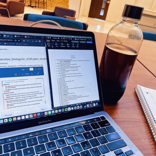
Day 92 • 100 Days of Productivity

i had my lecture exam for bio today and i don’t think I did bad but i think i could have done better tbh. but i did a lot of studying so i wonder how the rest of my group who didn’t did. i’m working on finishing random tasks and I’m starting to bullet journal in german to practice more. my oma is coming from berlin in may and i want to be able to talk to her more lol. anywho have a good day yall

🎶 verliebt - antilopen gang 🎶

[jemma--studies]

u know someone’s about to get dragged through the mud when an academic uses the phrase ‘it’s tempting to assume’

[jemma--studies]

4 March 2024

First day of thesis work aaaa!

It actually wasn't that exciting in terms of the lab work I got to do, but it was exciting in terms of... everything else lol. I did the first synthesis and left the whole thing to crystallize (thesis supervisor said to forget about the solutions - apparently, they crystallize better when you aren't thinking about them ahaha). The entire day was a great challenge for my social anxiety and I'm very happy with how I handled things :) I'm exhausted though. I think I'll sleep supremely well tonight

[jemma--studies]

[jemma--studies]

dark academia (sitting in one place so long the library's motion-sensitive lights have turned off)

[jemma--studies]

22.02.2024—very strange to be watching lectures again. so many notes to take

[jemma--studies]

me: *hears fresh academic gossip*

me the second I see my advisor:

[jemma--studies]

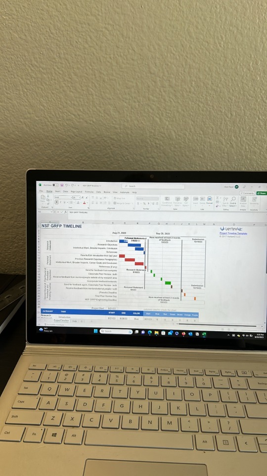
october 2nd, 2023

you ever make a plan..and then end up not following that plan at ALL? that is me with this NSF GRFP timeline that i made at the beginning of the semester.

i thought i'd have full, complete essays done by now and i don't LOL. and i'm supposed to send everything off for feedback to my PI tomorrow. so today is probably going to be a "binge writing"-esque type day. I still have like 2 paragraphs left for each document... we'll just see what happens. mind you, its due in a few weeks. so yeah thats my life.

this week's agenda

anatomy exam

booking conference stuff (registration, flights, etc - rip to my wallet)

[jemma--studies]

I come across a great site to learn coding, I don’t see a lot of people talking about it tho. (There is an app too!)

This site has python 101 for free (and many another, tho course from 102 and up aren’t free)

Its has a cute design and great at explaining the small details that some teachers don’t explain ✨

There is also many exercises in each chapter of the lessons.

You can check more about it from there official site ✨

Happy coding you all 🫶🏻

[jemma--studies]

Debug Help | Resources ✨

[jemma--studies]

Guys, I've managed to connect to my mongoDB database at last! Databases and express apps are kind of a new world to me tbh so I'm so excited to be learning all these new concepts!

My app is coming along ;) yay 🌱

[jemma--studies]

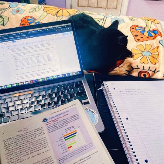
A big part of marine biology is quantitative math and statistics, so for anyone considering this as a career, just be prepared for that.

 It’s a good idea to learn to use a statistics program called “R.” It’s free and there are many plugins that scientists have made specifically for biology. It feels like programming, but there are lots of tutorials both within the program, and on Youtube.

This program will help you make sense of the data you collect, as well as visualize it.

[jemma--studies]

Multiple Linear Regression using R

Linear Regression

The relation between a dependent and an independent variable can be seen or predicted using linear regression models. When two or more independent variables are employed in a regression analysis, the model is referred to as a multiple regression model rather than a linear model.

Simple linear regression is a technique for predicting the value of one variable from the value of another. With linear regression, the relationship between the two variables is represented as a straight line.

In multiple regression, a dependent variable has a linear relationship with two or more independent variables. The dependent and independent variables may not follow a straight line if the relationship is non-linear.

When two or more variables are used to track a response, linear and non-linear regression are used. The non-linear regression is based on trial-and-error assumptions and is comparatively difficult to implement.

Multiple Linear Regression

Multiple linear regression is a statistical analysis technique that uses two or more factors to predict a variable’s outcome. It is also known as multiple regression and is an extension of linear regression. The dependent variable is the one that has to be predicted, and the factors that are used to forecast the value of the dependent variable are called independent or explanatory variables.

Analysts can use multiple linear regression to determine the model’s variance and the relative contribution of each independent variable. There are two types of multiple regression: linear and non-linear regression.

Multiple Regression Equation

The equation for multiple regression with three predictor variables (x) predicting variable y is as follows:

Y = B0 + B1 * X1 + B2 * X2 +B3 * X3

The beta coefficients are represented by the “B” values, which are the regression weights. They are the correlations between the predictor and the result variables.

Yi is predictable variable or dependent variable

B0 is the Y Intercept

B1 and B2 the regression coefficients represent the change in y as a function of a one-unit change in x1 and x2, respectively.

Multiple Linear Regression Assumptions

        I.            The Independent Variables are not Much Correlated

Multicollinearity, which occurs when the independent variables are highly correlated, should not be present in the data. This will make finding the specific variable that contributes to the variance in the dependent variable difficult.

   II.            Relationship Between Dependent and Independent Variables

Each independent variable has a linear relationship with the dependent variable. A scatterplot is constructed and checked for linearity to check the linear relationships. If the scatterplot relationship is non-linear, the data is transferred using statistical software or a non-linear regression is done.

III.            Observation Independence

The observations should be of each other, and the residual values should be independent. The Durbin Watson statistic works best for this.

Multiple Linear Regression in R

Analyzing the linear relationship between Stock Index Prices and Unemployment rate in the Economy.

Multiple linear regression can be done in a variety of methods, although statistical software is the most popular. R, a free, powerful, and easily accessible piece of software, is one of the most widely used. We’ll start by learning how to perform regression with R, then look at an example to make sure we understand everything.

Steps to Apply Multiple Linear Regression in R

Step 1: Data Collection

The data needed for the forecast is gathered and collected. The purpose is to use two independents

·         Unemployment Rate

·         Interest Rate

to forecast the stock index price (the dependent variable) of a fictional economy.

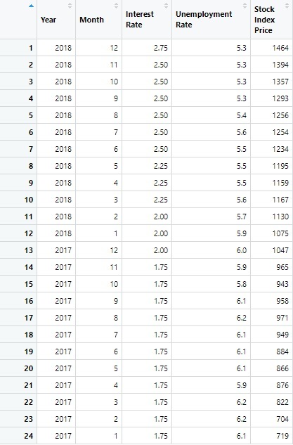
Step 2: Capturing the Data in R

Data Capturing using the code in R and Importing Excel file from save folder.

Step 3: Checking Data Linearity with R

It is critical to ensure that the dependent and independent variables have a linear relationship. Scatter plots or R code can be used to do this. Scatter plots are a quick technique to check for linearity. We need to make sure that various assumptions are met before using linear regression models. Most importantly, you must ensure that the dependent variable and the independent variable(s) have a linear relationship.

In this we’ll check the Linear Relationship exist between:

·         Stock Index Price (Dependent Variable) and Interest Rate (Independent Variable)

·         Stock Index Price (Dependent Variable) and Unemployment Rate (Independent Variable)

Below is the code that is used in R to plot the relations between the dependent variable that is Stock Index Price and Interest Rate.

From the Graph we can notice that there is Indeed a Linear relationship exist between the dependent variable Stock Index Price and Independent variable Interest Rate.

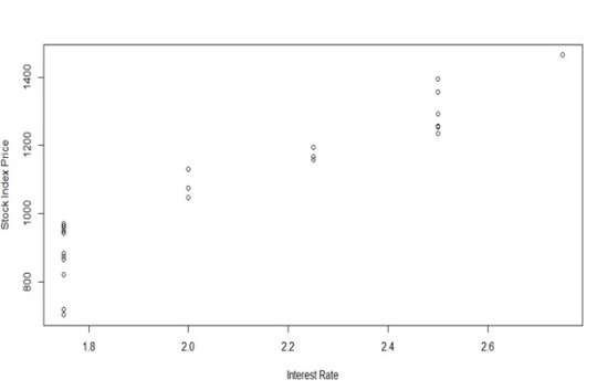
In can be specifically noted that When interest rates rise, the price of the stock index rises as well.

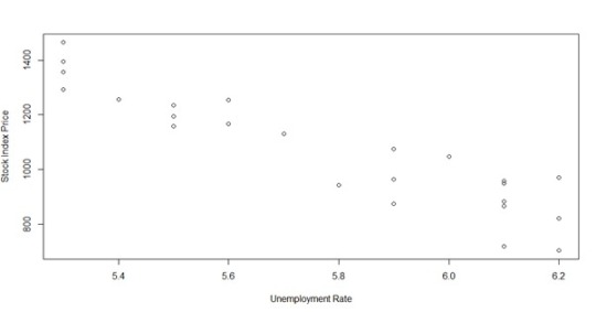
In the second scenario, we can plot the link between the Stock Index Price and the Unemployment Rate using the code below:

As you can see, the Stock Index Price and the Unemployment Rate have a linear relationship: when unemployment rates rise, the stock index price drops. we still have a linear correlation, although with a negative slope.

Step 4: Perform Multiple Linear Regression In R

To generate a set of coefficients, use code to conduct multiple linear regression in R. Template to perform Multiple Linear Regression in R is as below:

M1 <- lm (Dependent Variable ~ First Independent Variable + Second Independent Variable, Data= X)

Summary (M1)

Using the Template, the Code follows:

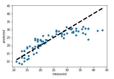
We will get the following summary if you execute the code in R:

The model’s residuals (‘Residuals’). The model fulfils heteroscedasticity assumptions if the residuals are roughly centered around zero and have similar spread on both sides (median -6.248, and min and max -158.2 and 118.8). The model’s regression coefficients ('Coefficients’).

To construct the multiple linear regression equation, utilize the coefficients from the summary as follows:

Stock Index Price = (Intercept) + (Interest Rate) X1* (Unemployment Rate) X2

Once you’ve entered the numbers from the summary: 

Stock Index Price = (1798.4) + (345.5) X1 * (-250.1) X2

Adjusted R-squared: Measures the model’s fit, with a higher number indicating a better fit.

The p-value is Pr(>|t|):  Statistical significance is defined as a p-value of less than 0.05.

Step 5: Make Predictions

 To predict the Stock Index Price from the collected Data it is noted that,

X1 <= Interest Rate = 1.5

X2 <= Unemployment Rate = 5.8

And when this data in equated into the regression Equation we obtain:

Stock Index Price = (1798.4) + (345.5) * (1.5) + (-250.1) * (5.8)

Stock Index Price = 866.066666

The Final Predicted data for the stock Index Price using Multiple Linear Regression is 866.07.

Conclusion

The stock market and our economy’s relationship frequently converge and diverges from one another. The gross domestic product, unemployment, inflation, and a slew of other indicators all represent the state of the economy. These trends are expected to show the economy and markets moving in lockstep in the long run.

When the unemployment rate is high, the Monetary Policy lowers the interest rate, which causes stock market prices to rise.

Unemployment increases often signify a drop in interest rates, which is good for stocks, as well as a drop in future corporate earnings and dividends, which is bad for stocks. Therefore, it is notable that Interest rate and Unemployment rate affect the stock market prices in the economy and have a linear relationship between the variables.

[jemma--studies]

R is one of the most widely used computer languages for statistical analysis and modelling. It is frequently used as a data science universal programming language. It is an open-source project and receives support from a community of passionate creators who work on new products. Various online websites offer R studio assignments help to comprehend the topics better. You may use R to do several statistical methods and derive them for free from various websites using power lines. For more information related to R studio assignment writing services visit My Assignment Services. 

[jemma--studies]

what the fuck is "dark academia" isnt real academia dark enough do you know what some of these fuckers woudl do for funding