jenifernguyen - Tumblr blog

jenifernguyen · 3 years

Text

Data Management and Visualization_Nguyen Thi Minh Ha_Week 4- Assignment

# -*- coding: utf-8 -*- """ Created on Thu Oct 7 00:37:40 2021

@author: hantm """

import pandas as pd import seaborn as sb import matplotlib.pyplot as plt

# load gapminder dataset data = pd.read_csv('gapminder.csv',low_memory=False) # lower-case all DataFrame column names data.columns = map(str.lower, data.columns) # bug fix for display formats to avoid run time errors pd.set_option('display.float_format', lambda x:'%f'%x)

# setting variables to be numeric data['suicideper100th'] = data['suicideper100th'].apply(pd.to_numeric, errors='coerce') data['breastcancerper100th'] = data['breastcancerper100th'].apply(pd.to_numeric, errors='coerce') data['hivrate'] = data['hivrate'].apply(pd.to_numeric, errors='coerce') data['employrate'] = data['employrate'].apply(pd.to_numeric, errors='coerce')

# display summary statistics about the data # print("Statistics for a Suicide Rate") # print(data['suicideper100th'].describe())

# subset data for a high suicide rate based on summary statistics sub = data[(data['suicideper100th']>12)] #make a copy of my new subsetted data sub_copy = sub.copy()

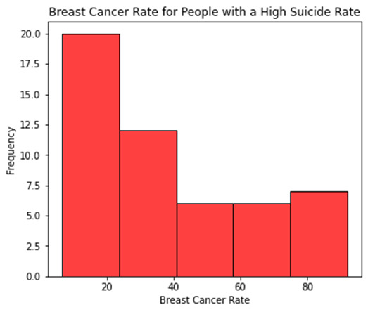
# Univariate graph for breast cancer rate for people with a high suicide rate plt.figure(1) sb.histplot(sub_copy["breastcancerper100th"], color="red", kde=False, bins=5) #sb.distplot(sub_copy["breastcancerper100th"].dropna(),kde=False) #sb.histplot(sub_copy["breastcancerper100th"], color="red", label="100% Equities", kde=True, stat="density", linewidth=0) #sb.histplot(sub_copy["hivrate"],kde=False) plt.xlabel('Breast Cancer Rate') plt.ylabel('Frequency') plt.title('Breast Cancer Rate for People with a High Suicide Rate') plt.show()

# Univariate graph for hiv rate for people with a high suicide rate plt.figure(2) #sb.distplot(sub_copy["hivrate"].dropna(),kde=False) #sb.histplot(sub_copy["hivrate"], color="red", label="100% Equities", kde=True, stat="density", linewidth=0) sb.histplot(sub_copy["hivrate"], color="red", label="100% Equities", kde=False, stat="density", linewidth=0) plt.xlabel('HIV Rate') plt.ylabel('Frequency') plt.title('HIV Rate for People with a High Suicide Rate') plt.show()

# Univariate graph for employment rate for people with a high suicide rate plt.figure(3) sb.histplot(sub_copy["employrate"], color="red", label="100% Equities", kde=True, stat="density", linewidth=0) plt.xlabel('Employment Rate') plt.ylabel('Frequency') plt.title('Employment Rate for People with a High Suicide Rate') plt.show()

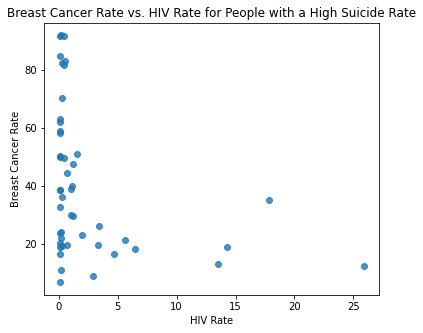
# Bivariate graph for association of breast cancer rate with HIV rate for people with a high suicide rate plt.figure(4) sb.regplot(x="hivrate",y="breastcancerper100th",fit_reg=False,data=sub_copy) plt.xlabel('HIV Rate') plt.ylabel('Breast Cancer Rate') plt.title('Breast Cancer Rate vs. HIV Rate for People with a High Suicide Rate') plt.show()

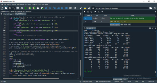
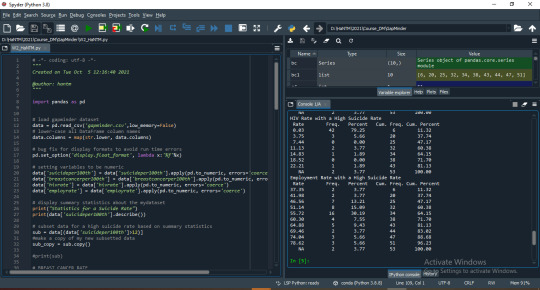
Please see my output file and code running in Python

#coursera

0 notes

jenifernguyen · 3 years

Text

Data Management and Visualization_Nguyen Thi Minh Ha_Week 3- Assignment

# -*- coding: utf-8 -*- """ Created on Thu Oct 7 00:37:40 2021

@author: hantm """

import pandas as pd import numpy as np import seaborn as sb import matplotlib.pyplot as plt

# display summary statistics about the data # print("Statistics for a Suicide Rate") # print(data['suicideper100th'].describe())

# subset data for a high suicide rate based on summary statistics sub = data[(data['suicideper100th']>12)] #make a copy of my new subsetted data sub_copy = sub.copy()

# Univariate graph for breast cancer rate for people with a high suicide rate plt.figure(1) sb.distplot(sub_copy["breastcancerper100th"].dropna(),kde=False) plt.xlabel('Breast Cancer Rate') plt.ylabel('Frequency') plt.title('Breast Cancer Rate for People with a High Suicide Rate')

# Univariate graph for hiv rate for people with a high suicide rate plt.figure(2) sb.distplot(sub_copy["hivrate"].dropna(),kde=False) plt.xlabel('HIV Rate') plt.ylabel('Frequency') plt.title('HIV Rate for People with a High Suicide Rate')

# Univariate graph for employment rate for people with a high suicide rate plt.figure(3) sb.distplot(sub_copy["employrate"].dropna(),kde=False) plt.xlabel('Employment Rate') plt.ylabel('Frequency') plt.title('Employment Rate for People with a High Suicide Rate')

# --------Output file -----------

#runfile('D:/HaNTM/2021/Course_DM/GapMinder/W3_HaNTM.py', #wdir='D:/HaNTM/2021/Course_DM/GapMinder')

Statistics for a Suicide Rate count 191.000000 mean 9.640839 std 6.300178 min 0.201449 25% 4.988449 50% 8.262893 75% 12.328551 max 35.752872 Name: suicideper100th, dtype: float64

Number of Breast Cancer Cases with a High Suicide Rate # of Cases Freq. Percent Cum. Freq. Cum. Percent (0.0, 23.0] 18 33.96 18 33.96 (23.0, 46.0] 15 28.30 33 62.26 (46.0, 69.0] 10 18.87 43 81.13 (69.0, 92.0] 8 15.09 51 96.23 nan 2 3.77 53 100.00

HIV Rate with a High Suicide Rate Rate Freq. Percent Cum. Freq. Cum. Percent 0% tile 18 33.96 18 33.96 25% tile 8 15.09 26 49.06 50% tile 11 20.75 37 69.81 75% tile 12 22.64 49 92.45 nan 4 7.55 53 100.00

Employment Rate with a High Suicide Rate Rate Freq. Percent Cum. Freq. Cum. Percent 1 10 18.87 10 18.87 2 24 45.28 34 64.15 3 5 9.43 39 73.58 4 13 24.53 52 98.11 5 1 1.89 53 100.00

#---------------------------------------------------------------------------------------

#p/s: Nguyen Thi Minh Ha (HaNTM)

#Data Management and Visualization

1 note · View note

jenifernguyen · 3 years

Text

Data Management and Visualization_Nguyen Thi Minh Ha_Week 2- Assignment 1

--------------------------------------------------------------------------------------------------------- Summary of Frequency Distributions ------------------------------------------------------ Question 1: What is a number of breast cancer cases associated with a high suicide rate? The high suicide rate is associated with the low number of breast cancer cases. ------------------------------------------------------ Question 2: How HIV rate is associated with a high suicide rate? The high suicide rate is associated with the low HIV rate.

------------------------------------------------------

Question 3: How employment rate is associated with a high suicide rate? The high suicide rate occurs at 55% of employment rate. -----------------------------------------------------------------------------------------------------------

# -*- coding: utf-8 -*- """ Created on Tue Oct 5 12:16:40 2021

@author: hantm """

import pandas as pd

# load gapminder dataset data = pd.read_csv('gapminder.csv',low_memory=False) # lower-case all DataFrame column names data.columns = map(str.lower, data.columns)

# bug fix for display formats to avoid run time errors pd.set_option('display.float_format', lambda x:'%f'%x)

# display summary statistics about the data print("Statistics for a Suicide Rate") print(data['suicideper100th'].describe())

# subset data for a high suicide rate based on summary statistics sub = data[(data['suicideper100th']>12)] #make a copy of my new subsetted data sub_copy = sub.copy()

#print(sub)

# BREAST CANCER RATE # frequency and percentage distritions for a number of breast cancer cases with a high suicide rate #print('frequency for a number of breast cancer cases with a high suicide rate') bc = sub_copy['breastcancerper100th'].value_counts(sort=False,bins=10) #print(bc) print('percentage for a number of breast cancer cases with a high suicide rate') pbc = sub_copy['breastcancerper100th'].value_counts(sort=False,bins=10,normalize=True)*100 #print(pbc)

# cumulative frequency and cumulative percentage for a number of breast cancer cases with a high suicide rate bc1=[] # Cumulative Frequency pbc1=[] # Cumulative Percentage cf=0 cp=0 for freq in bc: cf=cf+freq bc1.append(cf) pf=cf*100/len(sub_copy) pbc1.append(pf) #print('cumulative frequency for a number of breast cancer cases with a high suicide rate') #print(bc1) #print('cumulative percentage for a number of breast cancer cases with a high suicide rate') #print(pbc1)

print('Number of Breast Cancer Cases with a High Suicide Rate') fmt1 = '%s %7s %9s %12s %12s' fmt2 = '%5.2f %10.d %10.2f %10.d %12.2f' print(fmt1 % ('# of Cases','Freq.','Percent','Cum. Freq.','Cum. Percent'))

for i, (key, var1, var2, var3, var4) in enumerate(zip(bc.keys(),bc,pbc,bc1,pbc1)):

#print(key.left) print(fmt2 % (key.left, var1, var2, var3, var4))

fmt3 = '%5s %10s %10s %10s %12s' print(fmt3 % ('NA', '2', '3.77', '53', '100.00'))

# HIV RATE # frequency and percentage distritions for HIV rate with a high suicide rate #print('frequency for HIV rate with a high suicide rate') hc = sub_copy['hivrate'].value_counts(sort=False,bins=7) #print(hc)

#print('percentage for HIV rate with a high suicide rate') phc = sub_copy['hivrate'].value_counts(sort=False,bins=7,normalize=True)*100 #print(phc)

# cumulative frequency and cumulative percentage for HIV rate with a high suicide rate hc1=[] # Cumulative Frequency phc1=[] # Cumulative Percentage cf=0 cp=0 for freq in bc: cf=cf+freq hc1.append(cf) pf=cf*100/len(sub_copy) phc1.append(pf) #print('cumulative frequency for HIV rate with a high suicide rate') #print(hc1) #print('cumulative percentage for HIV rate with a high suicide rate') #print(phc1)

print('HIV Rate with a High Suicide Rate') fmt1 = '%5s %12s %9s %12s %12s' fmt2 = '%5.2f %10.d %10.2f %10.d %12.2f' print(fmt1 % ('Rate','Freq.','Percent','Cum. Freq.','Cum. Percent')) for i, (key, var1, var2, var3, var4) in enumerate(zip(hc.keys(),hc,phc,hc1,phc1)): print(fmt2 % (key.left, var1, var2, var3, var4)) fmt3 = '%5s %10s %10s %10s %12s' print(fmt3 % ('NA', '2', '3.77', '53', '100.00'))

# EMPLOYMENT RATE # frequency and percentage distritions for employment rate with a high suicide rate #print('frequency for employment rate with a high suicide rate') ec = sub_copy['employrate'].value_counts(sort=False,bins=10) #print(ec)

#print('percentage for employment rate with a high suicide rate') pec = sub_copy['employrate'].value_counts(sort=False,bins=10,normalize=True)*100 #print(pec)

# cumulative frequency and cumulative percentage for employment rate with a high suicide rate ec1=[] # Cumulative Frequency pec1=[] # Cumulative Percentage cf=0 cp=0 for freq in bc: cf=cf+freq ec1.append(cf) pf=cf*100/len(sub_copy) pec1.append(pf) #print('cumulative frequency for employment rate with a high suicide rate') #print(ec1) #print('cumulative percentage for employment rate with a high suicide rate') #print(pec1)

print('Employment Rate with a High Suicide Rate') fmt1 = '%5s %12s %9s %12s %12s' fmt2 = '%5.2f %10.d %10.2f %10.d %12.2f' print(fmt1 % ('Rate','Freq.','Percent','Cum. Freq.','Cum. Percent')) for i, (key, var1, var2, var3, var4) in enumerate(zip(ec.keys(),ec,pec,ec1,pec1)): print(fmt2 % (key.left, var1, var2, var3, var4)) fmt3 = '%5s %10s %10s %10s %12s' print(fmt3 % ('NA', '2', '3.77', '53', '100.00'))

#Output: runfile('D:/HaNTM/2021/Course_DM/GapMinder/W2_HaNTM.py', wdir='D:/HaNTM/2021/Course_DM/GapMinder')

Statistics for a Suicide Rate count 191.000000 mean 9.640839 std 6.300178 min 0.201449 25% 4.988449 50% 8.262893 75% 12.328551 max 35.752872 Name: suicideper100th, dtype: float64 Number of Breast Cancer Cases with a High Suicide Rate # of Cases Freq. Percent Cum. Freq. Cum. Percent 6.51 6 11.32 6 11.32 15.14 14 26.42 20 37.74 23.68 5 9.43 25 47.17 32.22 7 13.21 32 60.38 40.76 2 3.77 34 64.15 49.30 4 7.55 38 71.70 57.84 5 9.43 43 81.13 66.38 1 1.89 44 83.02 74.92 3 5.66 47 88.68 83.46 4 7.55 51 96.23 NA 2 3.77 53 100.00

HIV Rate with a High Suicide Rate Rate Freq. Percent Cum. Freq. Cum. Percent 0.03 42 79.25 6 11.32 3.75 3 5.66 20 37.74 7.44 0 0.00 25 47.17 11.13 2 3.77 32 60.38 14.83 1 1.89 34 64.15 18.52 0 0.00 38 71.70 22.21 1 1.89 43 81.13 NA 2 3.77 53 100.00

Employment Rate with a High Suicide Rate Rate Freq. Percent Cum. Freq. Cum. Percent 37.35 2 3.77 6 11.32 41.98 2 3.77 20 37.74 46.56 7 13.21 25 47.17 51.14 8 15.09 32 60.38 55.72 16 30.19 34 64.15 60.30 4 7.55 38 71.70 64.88 5 9.43 43 81.13 69.46 2 3.77 44 83.02 74.04 3 5.66 47 88.68 78.62 3 5.66 51 96.23 NA 2 3.77 53 100.00

#Data Management and Visualization

1 note · View note