#ggplot

[sophielovesbooks]

I've been refusing to get into ggplot for several years now and today is the day it's coming back to haunt me. 🥲

#phd #phd student #academia #i need to make pretty plots for my paper manuscript #and all the ones i've used in the past are soooo perfunctory #it's a terrible thing when you're suddenly forced to invest the effort you simply did not want to invest #R #ggplot #ggplot2

[queerforscience]

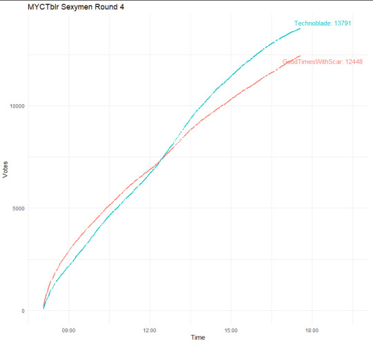
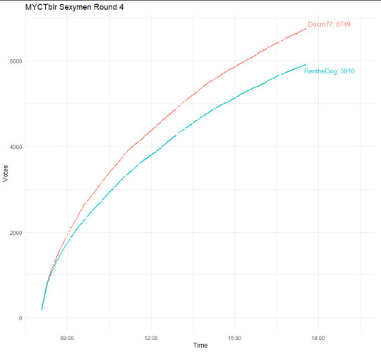
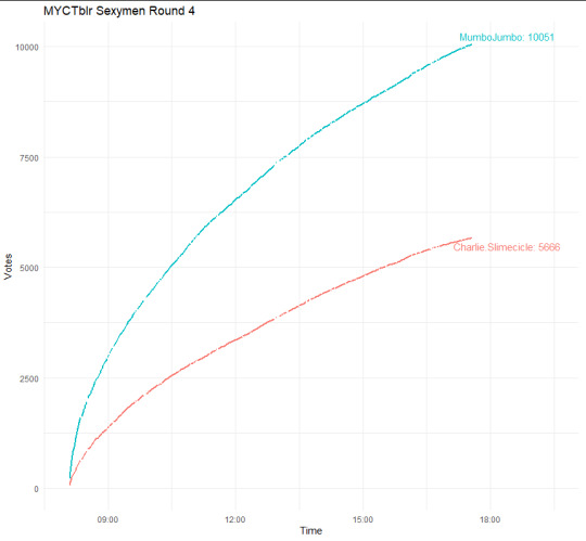
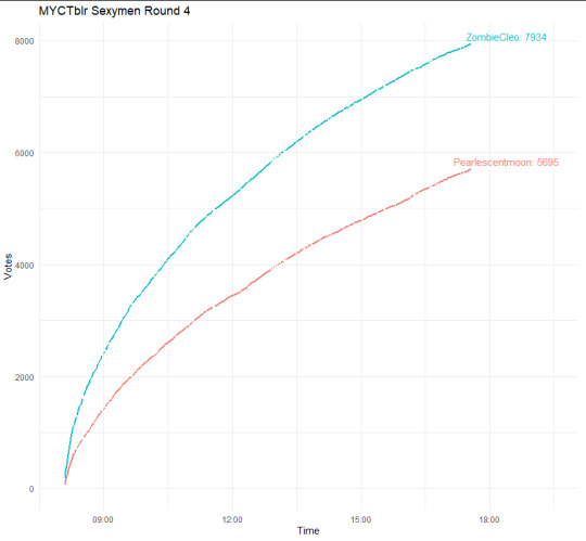
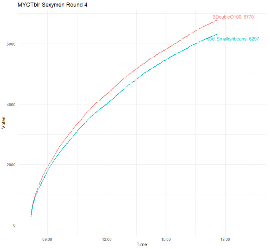
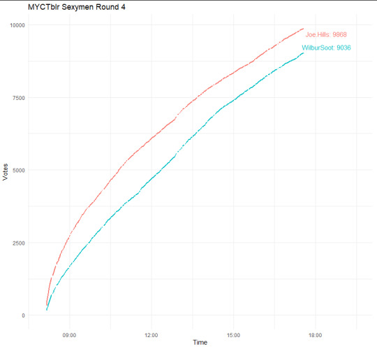
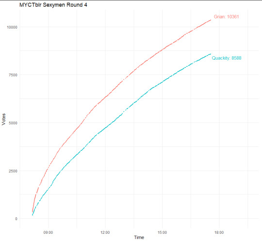
MCYTblr Sexymen Bracket Round 4 votes so far 👀

Code, in case there's somehow someone else invested in this who uses R lmao

Made with R, including the tidyverse and ggrepel packages.

Huge shoutout to @this-glittering-world for setting up the scraper for the current vote counts! The code is set up to pull their csvs so it updates every time you run it.

#mcytblrsexymen #mcytblr sexymen #ggplot #lmao #undescribed #I had to learn or remind myself how to do so many things with ggplot

[luridcomixofthenuit]

I would like u to know that no one has ever suffered as i have

#agrivoltaics #i am in pain #it hurts #r code #ggplot

[kathrynfknight]

Plot and the code to make it

#aphantasia #cogsci22 #raincloud plots #ggplot #R code

[ecosistemaglobal]

Gráficos en R con ggplot

que tipos de gráficos se pueden hacer con GGPLOT Vamos a ver que puede hacer ggplot2 para haer gráficos. PArece una técnica complicada porque visualmente ofrece basantes variedades, perro en realidad es mas sencillo de lo que parece. Mas bien, son muchas cosas sencillas que juntas , nos hacen creer que es dificil Latabla que usaremos es la…

View On WordPress

#ggplot #graficos

[drogouett]

GGplot.

#GGplot

[frontlinebicepsoftheninth]

hi everyone i went way too deep and used some code i had saved from a text mining course last year and ran some models to break down the emotional arcs of htn and ntn and now i have graphs and everything and i'm trying to write up an analysis but it is going to be so long. i may just post it on reddit and share the link. but now i wanna make a survey to test the model against reader opinions to see how accurate it is and if i do all that this may end up literally more time intensive than my final project for that class lmao

#like i love these books so much i WILLINGLY OPENED R #that program was the bane of my existence for a semester #also if anyone knows R and can help me figure out a problem with my graphing where the window of my x axis keeps randomly changing #even if i dont change anything in the code #i would be greatly appreciative #i had to update rstudio today so maybe it has something to do with that or maybe theres a newer ggplot package i need to install

[dodgebolts]

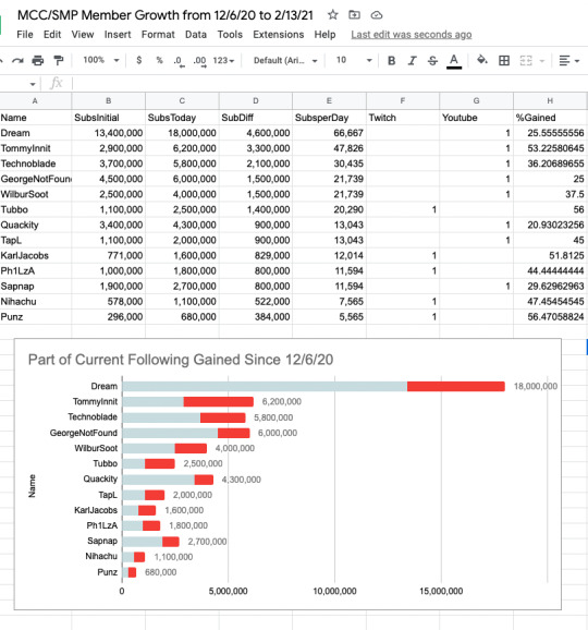
I went back and found some of the graphs they've all come so far :')

#I just have a ton of mcy.t data analysis content laying around on my computer and drives #idk where it all is though #I think the mc.c one is lost to the sands of time which sucks I really liked that one and had a lot of fun making it #color ramps in ggplot are fun to play with especially bc color was such an integral part of that one #it was cool and interactive too bc I was able to save it as an html :[ #man.

[oofuri2003]

do you think if abe didnt play baseball he would devote all of that mental scheming brain energy to like runescape or WoW. i just think if he didnt play baseball all of that brainpower would have to go somewhere and that somewhere would be MMOs

#like i know i said he sucks at video games and i believe that to be true #in the world where he plays baseball #but in the world where he DOESNT? well. #okay i swear to go i am going to do hw and tasks. i am typing ggplot patchwork into google to finish this assignment

[badolmen]

Spent two hours fighting tooth and nail to get like. 3 characters worth of code to work. I deserve a break <- still has 50% of the midterm to finish

#ra speaks #personal #my prof doesn’t like/use ggplots but I spent an hour and a half trying to get the standard bar plot function to do what I wanted #and ggplots has wayyyg more documentation/troubleshooting. figured it out in no time.

[rcsequr]

Ggplot rename x ticks

DOWNLOAD NOW Ggplot rename x ticks

#Ggplot rename x ticks manual

This then limits the arguments to relevant ones for the object. For example, if you use text, you can change every text element if you use title, you would change only the title text elements (plot/axes/legend titles) if you used axis.title, that would only change the axes titles, whereas would only change the x axis title, and so on!įor most arguments in theme(), you specify what kind of element you are changing ( element_line(), element_rect(), element_text(), or element_blank() to remove something). You can probably get a sense for what many of those might do, and as you can see there are often several versions so you can either apply a change to everything of that type or specific elements. This has a LOT of arguments that you can change here is the list from the documentation. The things changed within these built in themes can be accessed through the theme() function. These impact the colour of the plot, thickness and existence of gridlines, font details, legend position and more. There are several themes built into ggplot2, so you can easily use one of those to quickly achieve a look you are happy with. Scale_fill_discrete(labels = c("Adult", "Infant")) Mapping = aes(x = forcats::fct_infreq(Species), I’m also going to assign this to an object now so I can work on it without having to write the same lines repetitively. Bear in mind that if you have the forcats packaged loaded, you don’t need to specific the package in the function call, which makes it look a little less busy. Note that we also have to add in a label for the x axis otherwise we would get the unsightly forcats::fct_infreq(Species) as the label. The change comes in defining the x argument in aes(). The alternative is to transform your original data so your variable is a factor ordered by count, which is a bit cumbersome if the only reason you are doing it is for one plot. This is a quick and easy way using the forcats package, which doesn’t change your original data. This would be easier to interpret if the species were ordered by count (which would be more true if you had lots of species to compare). Scale_fill_discrete(labels = c("Adult", "Infant")) + Labs(y = "Count", title = "Number of hawks by species") + ggplot(data = hawks, mapping = aes(x = Species, fill = Age)) + The labels argument changes the labels.įor illustrative purposes, I’ve also used scale_y_continuous to change where the tick marks land (every 150 hawks) and spell out the labels. So here, we can change the labels on the legend with scale_fill_discrete(), because it relates to the fill aesthetic and it’s a categorical variable.

#Ggplot rename x ticks manual

The first part is scale, the second part is the aesthetic you are changing and the third part is whether it is discrete, continuous or manual (i.e. specified by you). There are a group of functions that cover these that all start with scale_*(). These are to do with the legend category labels and the labels on the axes ticks. However, there’s still text on there that we haven’t changed. There are other functions you can use that are more specialist, like xlab() and ylab() for the axes and ggtitle() for the title, but obviously those only cover those specific labels. Subtitle = "Red-tailed hawks were counted most often", Here’s an example with all of those things added. I like to use this function because you can use it to change the title, subtitle, caption or tags as well as the axes labels or other aesthetics. Starting with the labs() function, we can change a lot of the text.

DOWNLOAD NOW Ggplot rename x ticks

#Ggplot rename x ticks

[girinma]

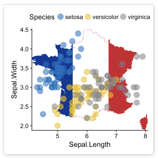
why would you ever want to make a graph like this

#i made a big pretty figure today so i had to once again look up how to use ggplot

[lovelymiral]

Plot two datasets on same graph r ggplot

Gggplot2 allows for the creation of dozens of geometric objects, transforms data with a variety of statistical analysis, and much more. This tutorial just barely sratches the surface of what is possible with this package. I won't offer any analysis of the resulting visualization since the data are fake, but the data and R script with comments are available here for those who would like to recreate this visualization themselves. The resulting chart looks something like this: Ggtitle("Income, Student Loans, Education Level, & Gender") "Education Level", shape = "Gender", size = "Commute Time (in minutes)") + Labs (x = "Student Loans (in dollars)", y = "Income (in dollars)", color = By including the alpha function in the geom layer, we avoid an unnecessary legend on the final visualization:įinally, add a title and change the labels for the axes and legends: Add opacity to the points to clearly see all points. Notice that some of the points are difficult to see due to overlapping. Ggplot(data, aes(x = student_loans, y = income, color = factor(education_level), shape = factor(gender), size = commute_time)) + There is no need to include factor, since time spent commuting is a continuous variable: We can size the points based on time spent commuting. Ggplot(data, aes(x = student_loans, y = income, color = factor(education_level), shape = factor(gender))) + Now, change the shape of the points to indicate gender: Ggplot(data, aes(x = student_loans, y = income, color = factor(education_level))) +įor discrete variables, such as education level or gender, it is important to include factor. We add color to the aesthetics of the plot: Let’s visually encode another variable by coloring the points based on education level. There are a variety of different geometric shapes available in ggplot2, such as geom_bar() for bar charts. Since we want to create a scatter plot we will use geom_point(). The next line adds a layer to the plot specifying the geometric shape to be used. In this case, we want to see student loan values on the x-axis and income on the y-axis. The first line specifies the dataset that we are using, followed by the aesthetics of the plot. Ggplot(data, aes(x = student_loans, y = income)) + The next step is to create a basic scatter plot comparing individuals’ student loans to their income: This creates a dataframe called data that has 200 observations and six variables. Now, read in the CSV file containing the sample data using the read.csv function:ĭata

#Plot two datasets on same graph r ggplot

[karmapiner]

Plot two datasets on same graph r ggplot

Plot two datasets on same graph r ggplot code#

Geom_point(data = pred_stats_per, aes(x=current_days_down_period, y=percent_incorrect*2), size = 3, color = 'black') + Geom_bar(data = pred_stats, aes(fill=pred_correct, x=current_days_down_period, y=count), position="stack", stat="identity") +

Plot two datasets on same graph r ggplot code#

My final adjustment was to scale each of the axes by using breaks = seq() as shown in the code below. By adding lty = 'Percent Incorrect' to aes of geom_line.Īdditionally I added scale_linetype('') to remove an unwanted title on the new legend. This luckily proved to be a simple addition. I was nearly done, but couldn’t help but try to add to the legend that the line represented the “Percent Incorrect”. This plot was showing exactly what I wanted, the relationship between the counts of correct and incorrect predictions as well as the percentage of incorrect predictions. These two steps created the secondary axes and made sure that the secondary y variable lined up properly. So in this case that code looked like this, when defining my y variable in both my geom_point() and geom_line(): You also need to do the inverse to your second y variable, because it is still lining up with the primary axis, it is not actually scaling off of the secondary axes. Scale_y_continuous(name = 'Count', sec.axis = sec_axis(~./2, name = 'Percent Incorrect')) You can see the syntax in the code below setting up the two axes. However, my counts on all plots totaled just over 200 so I made my secondary axis as half the primary. While these two are related, there wasn’t an easy operation to convert from the count to the percent. My secondary axis was a percentage of incorrect predictions, while the primary axis was showing the total count of predictions. In this case they are, although not as directly as is easily implemented.Īs mentioned above, when you create a secondary axis in ggplot2 it has to relate to the first axis. His words on the topic: “I agree that they can be useful when the axes are simple linear transformations of each other, but I don’t think they’re useful enough for me to spend hours to implement them.”ĭue to this, it is challenging to implement a dual axis plot in ggplot2, and is really only possible when the two axes are related to one another. Hadley Wickham, the creator of ggplot2, is not a fan of dual axis plots. Use the first plot with the counts and then overlay a line plot showing the percent of incorrect predictions. I decided that I would like to combine the two plots. I could use both plots, but I actually had this plot for multiple years and multiple models so using both would be a lot of plots in my notebook. I could just stick with this visualization, but showing that the number of predictions was decreasing over time was also important to me. Geom_bar(data = pred_stats, aes(fill=pred_correct, x=current_days_down_period, y=count), position="fill", stat="identity")+ Instead I see that my predictions actually became a little worse as time went on. This chart, shown below, does show how the previous plot was a little misleading. I decided to switch it to percentage instead of count. Subtitle = 'Prediction Performance by Current Days Not Flown Period', Labs(title = 'Random Forest Model Predicting on 2020', Geom_bar(data = pred_stats, aes(fill=pred_correct, x=current_days_down_period, y=count), position="stack", stat="identity")+ So while this chart is helpful in some ways, it is also a bit misleading, because the incorrect count is decreasing, but so is the total count. It appeared my predictions were improving over time as the number of incorrect predictions decreased, however the total number of predictions was also decreasing over time. The first visualization I came up with below, showed the counts of incorrect and correct predictions within the windows.

#Plot two datasets on same graph r ggplot

[longchecks]

Ggplot multipanel figure different legend different sizes

#GGPLOT MULTIPANEL FIGURE DIFFERENT LEGEND DIFFERENT SIZES PDF#

#GGPLOT MULTIPANEL FIGURE DIFFERENT LEGEND DIFFERENT SIZES SERIES#

#GGPLOT MULTIPANEL FIGURE DIFFERENT LEGEND DIFFERENT SIZES PDF#

Please create a single PDF file that contains all the original blot and gel images contained in the manuscript’s main figures and supplemental figures.

Please follow these instructions when preparing and submitting blot/gel data files: Whilst it is not necessary to provide original images at time of initial submission, we will require these files during the peer review process or before a manuscript can be accepted. If you have questions about these requirements please email us at Original images for blots and gelsĪuthors must provide the original, uncropped and minimally adjusted images supporting all blot and gel results reported in an article’s figures and supporting information files. The figure preparation guidelines that follow clarify PLOS ONE standards and requirements, and aim to ensure the integrity and scientific validity of blot/gel data reporting. The original images also provide additional information for readers about background within the experiment and the specificity of reagents used. The underlying data requirement is in place to ensure that the results are reported in a fully transparent manner, and that readers can verify results by reviewing the primary data in its original form. On the right, a second geom_point() layer is overlaid on the plot using small markers: this layer is associated with a different colour scale, used to indicate whether the vehicle has a 4-cylinder engine.The following requirements apply to any figures and supporting Information files that report blot or gel data. To illustrate this the plot on the left uses geom_point() to display a large marker for each vehicle make in the mpg data, with a single colour scale that maps to the year. 43 The ggnewscale::new_scale_colour() command acts as an instruction to ggplot2 to initialise a new colour scale: scale and guide commands that appear above the new_scale_colour() command will be applied to the first colour scale, and commands that appear below are applied to the second colour scale. Nevertheless, there are exceptions to this general rule, and it is possible to override this behaviour using the ggnewscale package. In general it is not advisable to map one aesthetic (e.g. colour) to multiple variables, and so by default ggplot2 does not allow you to “split” the colour aesthetic into multiple scales with separate legends. Splitting a legend is a much less common data visualisation task.

18.4.1 Indirectly referring to variables.

15.2.3 Map projections with coord_map().

15.2.2 Polar coordinates with coord_polar().

15.2.1 Transformations with coord_trans().

15.1.2 Flipping the axes with coord_flip().

15.1.1 Zooming into a plot with coord_cartesian().

13.4.1 Specifying the aesthetics in the plot vs. in the layers.

10.7.4 guide_coloursteps() / guide_colorsteps().

10.7.3 guide_colourbar() / guide_colorbar().

8.2 Arranging plots on top of each other.

4.4 Matching aesthetics to graphic objects.

4.2 Different groups on different layers.

#GGPLOT MULTIPANEL FIGURE DIFFERENT LEGEND DIFFERENT SIZES SERIES#

2.6.5 Time series with line and path plots.2.6.3 Histograms and frequency polygons.2.4 Colour, size, shape and other aesthetic attributes.1.3 How does ggplot2 fit in with other R graphics?.ggplot2: elegant graphics for data analysis.

#Ggplot multipanel figure different legend different sizes

[gurgaonproperty]

Pyramid Imperial Estate Deen Dayal Plots Sector 70A Gurgaon

Pyramid Imperial Estate Deen Dayal Plots Sector 70A Gurgaon

Pyramid Imperial Estate Deen Dayal Plots Sector 70A Gurgaon, The Project is Strategically found in Sector 70a Gurgaon on Golf Course Extension Road. Spread Over 5.38 acres of land of area with least 65% of Open Space. Imperial Estate society Comes Under Deen Dayal Jan Awas Yojna Projects Licence Details – Pyramid Imperial Estate DDJAY Plots Developer Name- PYRAMID INFRATECH PRIVATE…

View On WordPress

#ddjay plots in gurgaon #Imperial Estate #Imperial Estate Gurgaon #pyramid deen dayal plots #Pyramid Imperial Estate #pyramid Imperial Estate construction update #pyramid Imperial Estate plots #pyramid Imperial Estate plots for sale #pyramid Imperial Estate plots Gurgaon #pyramid Imperial Estate sector 35 Gurgaon #pyramid imperial plots Gurgaon #pyramid infratech #pyramid plot ggplot #Pyramid plots #pyramid plots Gurgaon #pyramid plots Gurgaon road #pyramid plots sector 70 gurgaon #pyramid plots sector 70a #upcoming ddjay plots in gurgaon