#linecolors

[mrcodings]

Click Here To Watch Full Tutorial

🔥🔥🔥🔥🔥🔥🔥🔥🔥🔥🔥🔥

MS Excel Tutorial Part-005 Cell Border | Border in Font Group | Line Style | Line Color | Draw Border | In Hindi

In this, we will learn the border options of Font Group in the Home tab of MS Excel. We will learn below given topics.

Borders of the Cell

Remove the border of the Cells

Set All side borders of the Cell

Set Thick Outside Border of Cell

Draw Border

Draw Border Grid

Difference between Draw Border and Draw Border Grid

Erase Border

Set or Change Border color i.e. Line Color

Set or Change Border Style i.e. Line Style

Draw Cross border in Cell

These all are very basic and very important topics in MS Excel. This option is very helpful while we formating content. This is the only video tutorial where you will find 100% practical examples. In this Hindi video tutorial, we create videos in such a way that anyone can easily understand the topic. Then also if you have any queries, please comment with us, and we will reply to you.

MsExcelPart005, #HomeTab, #FontGroup, #CellBorder, #BorderStyle, #LineColor, #DrawBorder, #DrawCrossBorder, #MrCoding, #MrCoding33, #BestMsExcelTutorial, #MsExcelTutorialInHindi

#Ms Excel Part 005 #Home Tab #Font Group #Cell Border #Border Style #Line Color #Draw Border #Draw Cross Border #Mr Coding #Mr Coding33 #Best Ms Excel Tutorial #Ms Excel Tutorial In Hindi

[frammmb]

Feu,

Encre de chine, crayon et feutre sur papier.

#feu #fire #voile #curtain #sail #colors #linedrawing #linecolors #contemporary drawing #art contemporain #artecontemporanea #francoisebeal

[nahubun]

happy (maybe) birthday phoenix! also since this is a day (technically 2 days since its midnight) late happy birthday to the phoenix wright original game!!! 

#sorry ive been so inactive ive been working on a video game!! more details 2 come soon #phoenix wright #narumitsu #wrightworth #trucy wright #miles edgeworth #ace attorney #pearl fey #maya fey #dick gumshoe #larry butz #i wish i knew how to color palette normally #i mean ig i sorta jst didnt wnt this 2 take longer than it already had so i rushed the coloring portion i have a draft where im fixing the #line density/linecolor/coloring and adding shading and more detail but idk if ill actually ever get it done #i think this is good enough! atleast i did it

[chzwareena]

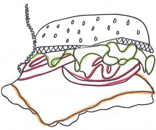
P E O N Y.

#botanic garden #linework #engraved #linetattoo #botanist #tattoos #engraving #linecolor #illustrator #botanical #peonyrose #peony #etching #etchingtattoo #lineart #colorwork #colortattoo #botanik #botanique #botany

[naptechlabs]

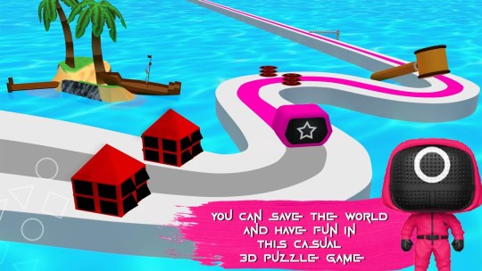
Line Color 3D Color Adventure Squid Game

Line Color 3D features a colorful world where players must race against the clock and save all of the color in this wonderful place before darkness takes over completely. Along the way, players will be able to collect coins which they can use at their own discretion for power-ups or other bonuses on future games!

#naptechlabs naptechgames linecolor coloradventure

[merlshmallow]

You’ve been blessed by Dima, @benaya-trash

#here you are #ignore the changing linecolor please i did weird stuff to the opacity #my art #olga #animation

[kamisaiyajin]

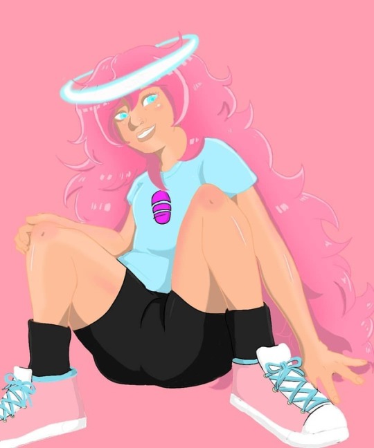
I thought about playing with the linecolor a bit. Hmm how does this look? _____________________________________ #artist #art #draw #drawing #angel #digitalart #archangel #azriel #amime #manga #oc https://www.instagram.com/p/BvBEmT_FTuw/?utm_source=ig_tumblr_share&igshid=gsdlzqreu7lk

#artist #art #draw #drawing #angel #digitalart #archangel #azriel #amime #manga #oc

[annapontoexe]

Transformações de Intensidade e Filtragem Espacial

1.      Realizar a limiarização de uma imagem usando Python e scikit-image.

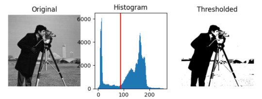
Uma limiarização de imagem é a transformação de uma imagem para binário, o que significa que ela ficará em preto e branco. Neste método, é “pesado” o histograma da imagem e a partir deste peso é removido o peso do lado mais pesado, até que os dois lados se equilibrem. Abaixo um exemplo de código:

import matplotlib.pyplot as plt from skimage import data from skimage.filters import threshold_otsu image = data.camera() thresh = threshold_otsu(image) binary = image > thresh fig, axes = plt.subplots(ncols=3, figsize=(8, 2.5)) ax = axes.ravel() ax[0] = plt.subplot(1, 3, 1) ax[1] = plt.subplot(1, 3, 2) ax[2] = plt.subplot(1, 3, 3, sharex=ax[0], sharey=ax[0]) ax[0].imshow(image, cmap=plt.cm.gray) ax[0].set_title('Original') ax[0].axis('off') ax[1].hist(image.ravel(), bins=256) ax[1].set_title('Histogram') ax[1].axvline(thresh, color='r') ax[2].imshow(binary, cmap=plt.cm.gray) ax[2].set_title('Thresholded') ax[2].axis('off') plt.show()

Exemplo de imagens:

Bibliografia:

https://pt.wikipedia.org/wiki/Limiarização_por_equilíbrio_do_histograma

https://scikit-image.org/docs/stable/auto_examples/developers/plot_threshold_li.html#sphx-glr-auto-examples-developers-plot-threshold-li-py

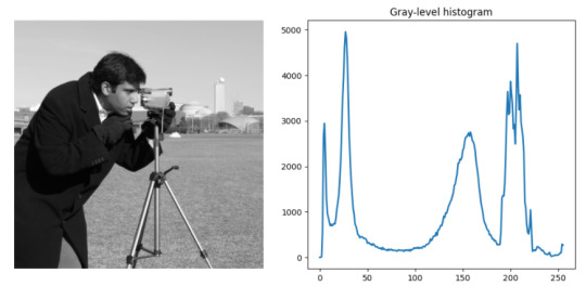
2.      Plotar o histograma de uma imagem tons de cinza usando Python, scikit-image e matplotlib.

O histograma de uma imagem em tons de cinza apresenta um gráfico resultante descritivo dos tons e frequência dos mesmos na imagem.

import numpy as np import matplotlib.pyplot as plt from skimage.util import img_as_ubyte from skimage import data from skimage.exposure import histogram noisy_image = img_as_ubyte(data.camera()) hist, hist_centers = histogram(noisy_image) fig, ax = plt.subplots(ncols=2, figsize=(10, 5)) ax[0].imshow(noisy_image, cmap=plt.cm.gray) ax[0].axis('off') ax[1].plot(hist_centers, hist, lw=2) ax[1].set_title('Gray-level histogram') plt.tight_layout()

Exemplo de imagem:

Bibliografia:

https://scikit-image.org/docs/stable/auto_examples/applications/plot_rank_filters.html#sphx-glr-auto-examples-applications-plot-rank-filters-py

3.      Plotar o histograma de uma imagem colorida (um histograma por canal de cor) usando Python, scikit-image e matplotlib.

""" * Python program to create a color histogram. * * Usage: python ColorHistogram.py <filename>"""import sysimport numpy as npimport skimage.colorimport skimage.iofrom matplotlib import pyplot as plt # read original image, in full color, based on command# line argumentimage = skimage.io.imread(fname='kodim23.png') # display the imageskimage.io.imshow(image)# tuple to select colors of each channel linecolors = ("red", "green", "blue")channel_ids = (0, 1, 2) # create the histogram plot, with three lines, one for# each colorplt.xlim([0, 256])for channel_id, c in zip(channel_ids, colors):    histogram, bin_edges = np.histogram(        image[:, :, channel_id], bins=256, range=(0, 256)    )    plt.plot(bin_edges[0:-1], histogram, color=c) plt.xlabel("Color value")plt.ylabel("Pixels") plt.show()

Bibliografia: https://datacarpentry.org/image-processing/05-creating-histograms/

4.      Equalizar o histograma de uma imagem usando Python e scikit-image.

import matplotlib import matplotlib.pyplot as plt import numpy as np from skimage import data, img_as_float from skimage import exposure matplotlib.rcParams['font.size'] = 8 def plot_img_and_hist(image, axes, bins=256):    """Plot an image along with its histogram and cumulative histogram.    """    image = img_as_float(image)    ax_img, ax_hist = axes    ax_cdf = ax_hist.twinx()    # Display image    ax_img.imshow(image, cmap=plt.cm.gray)    ax_img.set_axis_off()    # Display histogram    ax_hist.hist(image.ravel(), bins=bins, histtype='step', color='black')    ax_hist.ticklabel_format(axis='y', style='scientific', scilimits=(0, 0))    ax_hist.set_xlabel('Pixel intensity')    ax_hist.set_xlim(0, 1)    ax_hist.set_yticks([])    # Display cumulative distribution    img_cdf, bins = exposure.cumulative_distribution(image, bins)    ax_cdf.plot(bins, img_cdf, 'r')    ax_cdf.set_yticks([])    return ax_img, ax_hist, ax_cdf # Load an example image img = data.moon() # Contrast stretching p2, p98 = np.percentile(img, (2, 98)) img_rescale = exposure.rescale_intensity(img, in_range=(p2, p98)) # Equalization img_eq = exposure.equalize_hist(img) # Adaptive Equalization img_adapteq = exposure.equalize_adapthist(img, clip_limit=0.03) # Display results fig = plt.figure(figsize=(8, 5)) axes = np.zeros((2, 4), dtype=np.object) axes[0, 0] = fig.add_subplot(2, 4, 1) for i in range(1, 4):    axes[0, i] = fig.add_subplot(2, 4, 1+i, sharex=axes[0,0], sharey=axes[0,0]) for i in range(0, 4):    axes[1, i] = fig.add_subplot(2, 4, 5+i) ax_img, ax_hist, ax_cdf = plot_img_and_hist(img, axes[:, 0]) ax_img.set_title('Low contrast image') y_min, y_max = ax_hist.get_ylim() ax_hist.set_ylabel('Number of pixels') ax_hist.set_yticks(np.linspace(0, y_max, 5)) ax_img, ax_hist, ax_cdf = plot_img_and_hist(img_rescale, axes[:, 1]) ax_img.set_title('Contrast stretching') ax_img, ax_hist, ax_cdf = plot_img_and_hist(img_eq, axes[:, 2]) ax_img.set_title('Histogram equalization') ax_img, ax_hist, ax_cdf = plot_img_and_hist(img_adapteq, axes[:, 3]) ax_img.set_title('Adaptive equalization') ax_cdf.set_ylabel('Fraction of total intensity') ax_cdf.set_yticks(np.linspace(0, 1, 5)) # prevent overlap of y-axis labels fig.tight_layout() plt.show()

Bibliografia:

https://scikit-image.org/docs/stable/auto_examples/color_exposure/plot_equalize.html?highlight=histogram

5.      Detectar (concluir) que uma foto está subexposta ou que está superexposta, analisando o histograma.

Uma foto subexposta é quando o histograma apresenta a maior concentração de informações à esquerda do gráfico de exposição:

Uma foto superexposta é quando o histograma apresenta maior concentração no lado direito de seu histograma:

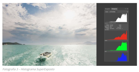
Bibliografia: https://criadoreslab.com.br/histograma-na-fotografia/

https://lightroombrasil.com.br/porque-fotografar-subexposto-e-melhor-que-superexposto/

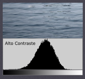
6.      Detectar (concluir) se uma imagem está com baixo contraste ou alto contraste, analisando o histograma.

É possível saber se uma imagem está com alto ou baixo contraste de acordo com a largura de seu histograma, por exemplo:

Um histograma como abaixo significa uma foto com baixo contraste, pois tem muitos pixels com basicamente as mesmas cores:

Já um histograma com alto contraste tem menos pixels, porém com muito mais cores distribuídas, assim seu gráfico fica mais largo:

Bibliografia:

https://www.cambridgeincolour.com/pt-br/tutoriais/histograms1.htm

[mmkumr]

Executing i3lock after suspend

Normally in i3wm tiling manager it doesn’t automatically lock the screen after suspend mode. For automating this process we can add the below line to our i3 config file:-

exec --no-startup-id xss-lock --transfer-sleep-lock -- lock --nofork

The word after --transfer-sleep-lock -- is name of the command which you want to run before system suspend (i.e. the word “lock”). I am using arch Linux. So, I have installed a package named as ‘i3lock-color’ from aur. I have also written one script for i3lock-color and stored it as executable.

i3lock-color script:-

#!/bin/sh

B='#00000000'  # blank

C='#ffffff22'  # clear ish

D='#ffffffcc'  # default

T='#ee00eeee'  # text

W='#880000bb'  # wrong

V='#bb00bbbb'  # verifying

i3lock \

--insidevercolor=$C   \

--ringvercolor=$V     \

\

--insidewrongcolor=$C \

--ringwrongcolor=$W   \

\

--radius=150          \

--insidecolor=$B      \

--ringcolor=$D        \

--linecolor=$B        \

--separatorcolor=$D   \

\

--verifcolor=$T        \

--wrongcolor=$T        \

--timecolor=$T        \

--datecolor=$T        \

--layoutcolor=$T      \

--keyhlcolor=$W       \

--bshlcolor=$W        \

\

--ignore-empty-password \

--blur 8              \

--clock               \

--indicator           \

--timestr="%l:%M:%S %p"  \

--datestr="%A, %m %Y" \

--screen 1            \

You can get more information by checking the man page of i3lock. After installing i3lock-color package.

[gamehayapkmod]

LineColor

LineColor

Game LineColor là dòng game Action

Giới thiệu LineColor

Colour Adventure is a fun colouring and brain training game in one! Tap and hold down to colour a path to new places and countries. But it’s not as simple as it looks! Color and paint the roads with the gelly by sliding on it! Go through the color lines of the road to become the first and have fun playing this fun and gelly color line cube 3d. Paint and color all the roads without rouching the abstacles on the road. Color all the lines on the roads with the colored gelly cube! color line cube 3d is one of the best games on the store. Hold your jelly cube on the road line to move the next level This game is a great line color game . In this gelly color line road game you can't jump. So watch out from any obstacles . Why you’ll love Colour Adventure: - Easy controls - Simple gameplay - Vibrant graphics - Lots of maps - Minimalist design Good luck

Download APK

Tải APK ([app_filesize]) #gamehayapk #gameandroid #gameapk #gameupdate

[chzwareena]

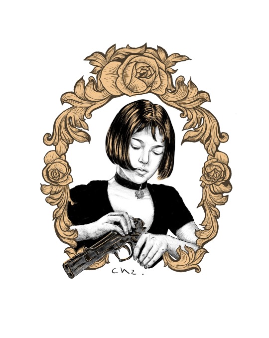
M A T H I L D A

#tattoodesign #tattoo #tattoos #illustrator #illustration #engravingtattoo #engraved #engraving #mathilda #etching #etchingtattoo #linecolor #linework #lineart #linetattoo #blacktattoo #blackwork

[sillyyouthdinosaur]

watchOS 6.2 add new color and gradients for Numerals and Gradient faces : AppleWatch *display:inline-block;vertical-align:middle.t9oUK2WY0d28lhLAh3N5qmargin-top:-23px._2KqgQ5WzoQRJqjjoznu22odisplay:inline-block;-ms-flex-negative:0;flex-shrink:0;position:relative._2D7eYuDY6cYGtybECmsxvE-ms-flex:1 1 auto;flex:1 1 auto;overflow:hidden;text-overflow:ellipsis._2D7eYuDY6cYGtybECmsxvE:hovertext-decoration:underline._19bCWnxeTjqzBElWZfIlJbfont-size:16px;font-weight:500;line-height:20px;display:inline-block._2TC7AdkcuxFIFKRO_VWis8margin-left:10px;margin-top:30px._2TC7AdkcuxFIFKRO_VWis8._35WVFxUni5zeFkPk7O4iiBmargin-top:35px._7kAMkb9SAVF8xJ3L53gcWdisplay:-ms-flexbox;display:flex;margin-bottom:8px._7kAMkb9SAVF8xJ3L53gcW>*-ms-flex:auto;flex:auto._1LAmcxBaaqShJsi8RNT-Vppadding:0 2px 0 4px;vertical-align:middle.nEdqRRzLEN43xauwtgTmjpadding-right:4px._3_HlHJ56dAfStT19Jgl1bFpadding-left:16px;padding-right:4px._2QZ7T4uAFMs_N83BZcN-Emfont-family:Noto Sans,Arial,sans-serif;font-size:14px;font-weight:400;line-height:18px;display:-ms-flexbox;display:flex;-ms-flex-flow:row nowrap;flex-flow:row nowrap._19sQCxYe2NApNbYNX5P5-Lcursor:default;height:16px;margin-right:8px;width:16px._3XFx6CfPlg-4Usgxm0gK8Rfont-size:16px;font-weight:500;line-height:20px._34InTQ51PAhJivuc_InKjJcolor:var(--newCommunityTheme-actionIcon)._29_mu5qI8E1fq6Uq5koje8font-size:12px;font-weight:500;line-height:16px;display:inline-block;word-break:break-word._2BY2-wxSbNFYqAy98jWyTCmargin-top:10px._3sGbDVmLJd_8OV8Kfl7dVvfont-family:Noto Sans,Arial,sans-serif;font-size:14px;font-weight:400;line-height:21px;margin-top:8px;word-wrap:break-word._1qiHDKK74j6hUNxM0p9ZIpmargin-top:12px._1eMniuqQCoYf3kOpyx83Jjdisplay:block;width:100%;margin-bottom:8px._326PJFFRv8chYfOlaEYmGt,.Jy6FIGP1NvWbVjQZN7FHAdisplay:block;width:100%;font-size:14px;font-weight:700;letter-spacing:.5px;line-height:32px;text-transform:uppercase;padding:0 16px.Jy6FIGP1NvWbVjQZN7FHAmargin-top:11px._1cDoUuVvel5B1n5wa3K507display:block;padding:0 16px;width:100%;font-size:14px;font-weight:700;letter-spacing:.5px;line-height:32px;text-transform:uppercase;margin-top:11px;text-transform:unset._2_w8DCFR-DCxgxlP1SGNq5margin-right:4px;vertical-align:middle._1aS-wQ7rpbcxKT0d5kjrbhborder-radius:4px;display:inline-block;padding:4px._2cn386lOe1A_DTmBUA-qSMborder-top:1px solid var(--newCommunityTheme-widgetColors-lineColor);margin-top:10px._2Zdkj7cQEO3zSGHGK2XnZvdisplay:inline-block.wzFxUZxKK8HkWiEhs0tyEfont-size:12px;font-weight:700;line-height:16px;color:var(--newCommunityTheme-button);cursor:pointer;text-align:left;margin-top:2px._3R24jLERJTaoRbM_vYd9v0._3R24jLERJTaoRbM_vYd9v0._3R24jLERJTaoRbM_vYd9v0display:none._38lwnrIpIyqxDfAF1iwhcVbackground-color:var(--newRedditTheme-line);border:none;height:1px;margin:16px 0.yobE-ux_T1smVDcFMMKFvfont-size:16px;font-weight:500;line-height:20px._2DVpJZAGplELzFy4mB0epQmargin-top:8px._2DVpJZAGplELzFy4mB0epQ .x1f6lYW8eQcUFu0VIPZzbcolor:inherit._2DVpJZAGplELzFy4mB0epQ svg.LTiNLdCS1ZPRx9wBlY2rDfill:inherit;padding-right:8px._2DVpJZAGplELzFy4mB0epQ ._18e78ihYD3tNypPhtYISq3font-family:Noto Sans,Arial,sans-serif;font-size:14px;font-weight:400;line-height:18px;color:inherit…

[kinkimken]

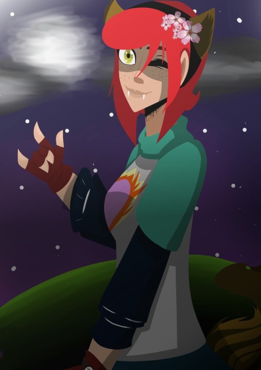
Pos! Estaba practicando el LineColor y pos, aqui esta :3 espero que os guste nwn

[mellau-expressive]

CHEEZ

#cheese #cheeseburger #burger #line #lineart #linecolor #black and color #art #trendy #fashion #sesame #bun #lettuce #tomato #food #design #mellau