#mathematical models
Text
How Much of the World Is It Possible to Model? Mathematical Models Power Our Civilization—But They Have Limits.
— By Dan Rockmore | January 15, 2024
Illustration by Petra Péterffy
It’s Hard For a Neurosurgeon to Navigate a Brain. A key challenge is gooeyness. The brain is immersed in cerebrospinal fluid; when a surgeon opens the skull, pressure is released, and parts of the brain surge up toward the exit while gravity starts pulling others down. This can happen with special force if a tumor has rendered the skull overstuffed. A brain can shift by as much as an inch during a typical neurosurgery, and surgeons, who plan their routes with precision, can struggle as the territory moves.
In the nineteen-nineties, David Roberts, a neurosurgeon, and Keith Paulsen, an engineer, decided to tackle this problem by building a mathematical model of a brain in motion. Real brains contain billions of nooks and crannies, but their model wouldn’t need to include them; it could be an abstraction encoded in the language of calculus. They could model the brain as a simple, sponge-like object immersed in a flow of fluid and divided into compartments. Equations could predict how the compartments would move with each surgical action. The model might tell surgeons to make the first cut a half inch to the right of where they’d planned to start, and then to continue inward at an angle of forty-three degrees rather than forty-seven.
Roberts and Paulsen designed their model on blackboards at Dartmouth College. Their design had its first clinical test in 1998. A thirty-five-year-old man with intractable epilepsy required the removal of a small tumor. He was anesthetized, his skull was cut open, and his brain began to move. The model drew on data taken from a preoperative MRI scan, and tracked the movement of certain physical landmarks during the surgery; in this way, the real and predicted topography of the exposed brain could be compared, and the new position of the tumor could be predicted. “The agreement between prediction and reality was amazing,” Roberts recalled recently.
Today, descendents of the Roberts and Paulsen model are routinely used to plan neurosurgeries. Modelling, in general, is now routine. We model everything, from elections to economics, from the climate to the coronavirus. Like model cars, model airplanes, and model trains, mathematical models aren’t the real thing—they’re simplified representations that get the salient parts right. Like fashion models, model citizens, and model children, they’re also idealized versions of reality. But idealization and abstraction can be forms of strength. In an old mathematical-modelling joke, a group of experts is hired to improve milk production on a dairy farm. One of them, a physicist, suggests, “Consider a spherical cow.” Cows aren’t spheres any more than brains are jiggly sponges, but the point of modelling—in some ways, the joy of it—is to see how far you can get by using only general scientific principles, translated into mathematics, to describe messy reality.
To be successful, a model needs to replicate the known while generalizing into the unknown. This means that, as more becomes known, a model has to be improved to stay relevant. Sometimes new developments in math or computing enable progress. In other cases, modellers have to look at reality in a fresh way. For centuries, a predilection for perfect circles, mixed with a bit of religious dogma, produced models that described the motion of the sun, moon, and planets in an Earth-centered universe; these models worked, to some degree, but never perfectly. Eventually, more data, combined with more expansive thinking, ushered in a better model—a heliocentric solar system based on elliptical orbits. This model, in turn, helped kick-start the development of calculus, reveal the law of gravitational attraction, and fill out our map of the solar system. New knowledge pushes models forward, and better models help us learn.
Predictions about the universe are scientifically interesting. But it’s when models make predictions about worldly matters that people really pay attention.We anxiously await the outputs of models run by the Weather Channel, the Fed, and fivethirtyeight.com. Models of the stock market guide how our pension funds are invested; models of consumer demand drive production schedules; models of energy use determine when power is generated and where it flows. Insurers model our fates and charge us commensurately. Advertisers (and propagandists) rely on A.I. models that deliver targeted information (or disinformation) based on predictions of our reactions.
But it’s easy to get carried away—to believe too much in the power and elegance of modelling. In the nineteen-fifties, early success with short-term weather modelling led John von Neumann, a pioneering mathematician and military consultant, to imagine a future in which militaries waged precision “climatological warfare.” This idea may have seemed mathematically plausible at the time; later, the discovery of the “butterfly effect”—when a butterfly flaps its wings in Tokyo, the forecast changes in New York—showed it to be unworkable. In 2008, financial analysts thought they’d modelled the housing market; they hadn’t. Models aren’t always good enough. Sometimes the phenomenon you want to model is simply unmodellable. All mathematical models neglect things; the question is whether what’s being neglected matters. What makes the difference? How are models actually built? How much should we trust them, and why?
Mathematical Modelling Began With Nature: the goal was to predict the tides, the weather, the positions of the stars. Using numbers to describe the world was an old practice, dating back to when scratchings on papyrus stood for sheaves of wheat or heads of cattle. It wasn’t such a leap from counting to coördinates, and to the encoding of before and after. Even early modellers could appreciate what the physicist Eugene Wigner called “the unreasonable effectiveness of mathematics.” In 1963, Wigner won the Nobel Prize for developing a mathematical framework that could make predictions about quantum mechanics and particle physics. Equations worked, even in a subatomic world that defied all intuition.
Models of nature are, in some ways, pure. They’re based on what we believe to be immutable physical laws; these laws, in the form of equations, harmonize with both historical data and present-day observation, and so can be used to make predictions. There’s an admirable simplicity to this approach. The earliest climate models, for example, were essentially ledgers of data run through equations based on fundamental physics, including Newton’s laws of motion. Later, in the nineteen-sixties, so-called energy-balance models described how energy was transferred between the sun and the Earth: The sun sends energy here, and about seventy per cent of it is absorbed, with the rest reflected back. Even these simple models could do a good job of predicting average surface temperature.
Averages, however, tell only a small part of the story. The average home price in the United States is around five hundred thousand dollars, but the average in Mississippi is a hundred and seventy-one thousand dollars, and in the Hamptons it’s more than three million dollars. Location matters. In climate modelling, it’s not just the distance from the sun that’s important but what’s on the ground—ice, water (salty or not), vegetation, desert. Energy that’s been absorbed by the Earth warms the surface and then radiates up and out, where it can be intercepted by clouds, or interact with chemicals in different layers of the atmosphere, including the greenhouse gases—carbon dioxide, methane, and nitrous oxide. Heat differentials start to build, and winds develop. Moisture is trapped and accumulates, sometimes forming rain, snowflakes, or hail. Meanwhile, the sun keeps shining—an ongoing forcing function that continually pumps energy into the system.
Earth-system models, or E.S.M.s, are the current state of the art in combining all these factors. E.S.M.s aim for high spatial and temporal specificity, predicting not only temperature trends and sea levels but also changes in the sizes of glaciers at the North Pole and of rain forests in Brazil. Particular regions have their own sets of equations, which address factors such as the chemical reactions that affect the composition of the ocean and air. There are thousands of equations in an E.S.M., and they affect one another in complicated couplings over hundreds, even thousands, of years. In theory, because the equations are founded on the laws of physics, the models should be reliable despite the complexity. But it’s hard to keep small errors from creeping in and ramifying—that’s the butterfly effect. Applied mathematicians have spent decades figuring out how to quantify and sometimes ameliorate butterfly effects; recent advances in remote sensing and data collection are now helping to improve the fidelity of the models.
How do we know that a giant model works? Its outputs can be compared to historical data. The 2022 Assessment Report from the Intergovernmental Panel on Climate Change shows remarkable agreement between the facts and the models going back two thousand years. The I.P.C.C. uses models to compare two worlds: a “natural drivers” world, in which greenhouse gases and particulate matter come from sources such as volcanoes, and a “human and natural” world, which includes greenhouse gases we’ve created. The division helps with interpretability. One of the many striking figures in the I.P.C.C. report superimposes plots of increases in global mean temperature over time, with and without the human drivers. Until about 1940, the two curves dance around the zero mark, tracking each other, and also the historical record. Then the model with human drivers starts a steady upward climb that continues to hew to the historical record. The purely natural model continues along much like before—an alternate history of a cooler planet. The models may be complicated, but they’re built on solid physics-based foundations. They work.
Of Course, there are many things we want to model that aren’t quite so physical. The infectious-disease models with which we all grew familiar in 2020 and 2021 used physics, but only in an analogical way. They can be traced back to Ronald Ross, an early-twentieth-century physician. Ross developed equations that could model the spread of malaria; in a 1915 paper, he suggested that epidemics might be shaped by the same “principles of careful computation which have yielded such brilliant results in astronomy, physics, and mechanics.” Ross admitted that his initial idea, which he called a “Theory of Happenings,” was fuelled more by intuition than reality, but, in a subsequent series of papers, he and Hilda Hudson, a mathematician, showed how real data from epidemics could harmonize with their equations.
In the nineteen-twenties and thirties, W.O. Kermack and A.G. McKendrick, colleagues at the Royal College of Physicians, in Edinburgh, took the work a step further. They were inspired by chemistry, and analyzed human interactions according to the chemical principle of mass action, which relates the rate of reaction between two reagents to their relative densities in the mix. They exchanged molecules for people, viewing a closed population in a pandemic as a reaction unfolding between three groups: Susceptibles (“S”), Infecteds (“I”), and Recovereds (“R”). In their simple “S.I.R. model”, “S”s become “I”s at a rate proportional to the chance of their interactions; “I”s eventually become “R”s at a rate proportional to their current population; and “R”s, whether dead or immune, never get sick again. The most important question is whether the “I” group is gaining or losing members. If it’s gaining more quickly than it’s losing, that’s bad—it’s what happens when a covid wave is starting.
Differential equations model how quantities change over time. The ones that come out of an S.I.R. model are simple, and relatively easy to solve. (They’re a standard example in a first applied-math course.) They produce curves, representing the growth and diminishment of the various populations, that will look instantly familiar to anyone who lived through covid. There are lots of simplifying assumptions—among them, constant populations and unvarying health responses—but even in its simplest form, an S.I.R. model gets a lot right. Data from real epidemics shows the characteristic “hump” that the basic model produces—the same curve that we all worked to “flatten” when covid-19 first appeared. The small number of assumptions and parameters in an S.I.R. model also has the benefit of suggesting actionable approaches to policymakers. It’s obvious, in the model, why isolation and vaccines will work.
The challenge comes when we want to get specific, so that we can more rationally and quickly allocate resources during a pandemic. So we doubled down on the modelling. As the covid crisis deepened, an outbreak of modelling accompanied the outbreak of the disease; many of the covid-specific models supported by the C.D.C. used an engine that featured a variation of the S.I.R. model. Many subdivided S.I.R.’s three groups into smaller ones. A model from a group at the University of Texas at Austin, for instance, divided the U.S. into two hundred and seventeen metro areas, segmenting their populations by age, risk factors, and a host of other characteristics. The model created local, regional, and national forecasts using cell-phone data to track mobility patterns, which reflected unprecedented changes in human behavior brought about by the pandemic.
S.I.R.s are one possible approach, and they occupy one end of a conceptual spectrum; an alternative called curve fitting is at the other. The core idea behind curve fitting is that, in most pandemics, the shape of the infection curve has a particular profile—one that can be well-approximated by gluing together a few basic kinds of mathematical shapes, each the output of a well-known mathematical function. The modeller is then more driven by practicalities than principles, and this has its own dangers: a pandemic model built using curve fitting looks like a model of disease trajectory, but the functions out of which it’s built may not be meaningful in epidemiological terms.
In the early stages of the pandemic, curve fitting showed promise, but as time went on it proved to be less effective. S.I.R.-based models, consistently updated with mortality and case data, ruled the day. But only for so long. Back in the nineteen-twenties, Kermack and McKendrick warned that their model was mainly applicable in an equilibrium setting—that is, in circumstances that didn’t change. But the covid pandemic rarely stood still. Neither people nor the virus behaved as planned. sars-CoV-2 mutated rapidly in a shifting landscape affected by vaccines. The pandemic was actually several simultaneous pandemics, interacting in complex ways with social responses. In fact, recent research has shown that a dramatic event like a lockdown can thwart the making of precise long-term predictions from S.I.R.-based models, even assuming perfect data collection. In December, 2021, the C.D.C. abruptly shut down its covid-19 case-forecast project, citing “low reliability.” They noted that “more reported cases than expected fell outside the forecast prediction intervals for extended periods of time.”
These kinds of failures, both in theory and practice, speak at least in part to the distance of the models from the phenomena they are trying to model. “Art is the lie that makes us realize the truth,” Picasso once said; the same could be said of mathematical modelling. All models reflect choices about what to include and what to leave out. We often attribute to Einstein the notion that “models should be as simple as possible, but not simpler.” But, elegance can be a trap—one that is especially easy to fall into when it dovetails with convenience. The covid models told a relatively simple and elegant story—a story that was even useful, inasmuch as it inspired us to flatten the curve. But, if what we needed was specific predictions, the models may have been too far from the truth of how covid itself behaved while we were battling it. Perhaps the real story was both bigger and smaller—a story about policies and behaviors interacting at the level of genomes and individuals. However much, we might wish for minimalism, our problems could require something baroque. That doesn’t mean that a pandemic can’t be modelled faithfully and quickly with mathematics. But we may be still looking for the techniques and data sources we need to accomplish it.
Formal Mathematical Election Forecasting is usually said to have begun in 1936, when George Gallup correctly predicted the outcome of the Presidential election. Today, as then, most election forecasting has two parts: estimating the current sentiment in the population, and then using that estimate to predict the outcome. It’s like weather prediction for people—at least in spirit. You want to use today’s conditions to predict how things will be on Election Day.
The first part of the process is usually accomplished through polling. Ideally, you can estimate the proportions of support in a population by asking a sample of people whom they would vote for if the election were to take place at that moment. For the math to work, pollsters need a “random sample.” This would mean that everyone who can vote in the election is equally likely to be contacted, and that everyone who is contacted answers truthfully and will act on their response by voting. These assumptions form the basis of mathematical models based on polling. Clearly, there is room for error. If a pollster explicitly—and statistically—accounts for the possibility of error, they get to say that their poll is “scientific.” But even with the best of intentions, true random sampling is difficult. The “Dewey Defeats Truman” debacle, from 1948, is generally attributed to polls conducted more for convenience than by chance.
Polling experts are still unsure about what caused so many poor predictions ahead of the 2016 and 2020 elections. (The 2020 predictions were the least accurate in forty years.) One idea is that the dissonance between the predicted (large) and actual (small) margin of victory for President Biden over Donald Trump was due to the unwillingness of Trump supporters to engage with pollsters. This suggests that cries of fake polling can be self-fulfilling, insofar as those who distrust pollsters are less likely to participate in polls. If the past is any indication, Republicans may continue to be more resistant to polling than non-Republicans. Meanwhile, pre-election polling has obvious limitations. It’s like using today’s temperature as the best guess for the temperature months from now; this would be a lousy approach to climate modelling, and it’s a lousy approach to election forecasting, too. In both systems, moreover, there is feedback: in elections, it comes from the measurements themselves, and from their reporting, which can shift (polled) opinion.
Despite these ineradicable sources of imprecision, many of today’s best election modellers try to embrace rigor. Pollsters have long attributed to their polls a proprietary “secret sauce,” but conscientious modellers are now adhering to the evolving standard of reproducible research and allowing anyone to look under the hood. A Presidential-forecast model created by Andrew Gelman, the statistician and political scientist, and G. Elliott Morris, a data journalist, that was launched in the summer of 2020 in The Economist, is especially instructive. Gelman and Morris are not only open about their methods but even make available the software and data that they use for their forecasting. Their underlying methodology is also sophisticated. They bring in economic variables and approval ratings, and link that information back to previous predictions in time and space, effectively creating equations for political climate. They also integrate data from different pollsters, accounting for how each has been historically more or less reliable for different groups of voters.
But as scientific as all this sounds, it remains hopelessly messy: it’s a model not of a natural system but of a sentimental one. In his “Foundation” novels, the writer Isaac Asimov imagined “psychohistory,” a discipline that would bring the rigor of cause and effect to social dynamics through equations akin to Newton’s laws of motion. But psychohistory is science fiction: in reality, human decisions are opaque, and can be dramatically influenced by events and memes that no algorithm could ever predict. Sometimes, moreover, thoughts don’t connect to actions. (“I can calculate the motion of heavenly bodies but not the madness of people,” Newton wrote.) As a result, even though election models use mathematics, they are not actually mathematical, in the mechanistic way of a planetary or even molecular model. They are fundamentally “statistical”—a modifier that’s both an adjective and a warning label. They encode historical relationships between numbers, and then use the historical records of their change as guidance for the future, effectively looking for history to repeat itself. Sometimes it works—who hasn’t, from time to time, “also liked” something that a machine has offered up to you based on your past actions? Sometimes, as in 2016 and 2020, it doesn’t.
Recently, statistical modelling has taken on a new kind of importance as the engine of artificial intelligence—specifically in the form of the deep neural networks that power, among other things, large language models, such as OpenAI’s G.P.T.s. These systems sift vast corpora of text to create a statistical model of written expression, realized as the likelihood of given words occurring in particular contexts. Rather than trying to encode a principled theory of how we produce writing, they are a vertiginous form of curve fitting; the largest models find the best ways to connect hundreds of thousands of simple mathematical neurons, using trillions of parameters.They create a vast data structure akin to a tangle of Christmas lights whose on-off patterns attempt to capture a chunk of historical word usage. The neurons derive from mathematical models of biological neurons originally formulated by Warren S. McCulloch and Walter Pitts, in a landmark 1943 paper, titled “A Logical Calculus of the Ideas Immanent in Nervous Activity.” McCulloch and Pitts argued that brain activity could be reduced to a model of simple, interconnected processing units, receiving and sending zeros and ones among themselves based on relatively simple rules of activation and deactivation.
The McCulloch-Pitts model was intended as a foundational step in a larger project, spearheaded by McCulloch, to uncover a biological foundation of psychiatry. McCulloch and Pitts never imagined that their cartoon neurons could be trained, using data, so that their on-off states linked to certain properties in that data. But others saw this possibility, and early machine-learning researchers experimented with small networks of mathematical neurons, effectively creating mathematical models of the neural architecture of simple brains, not to do psychiatry but to categorize data. The results were a good deal less than astonishing. It wasn’t until vast amounts of good data—like text—became readily available that computer scientists discovered how powerful their models could be when implemented on vast scales. The predictive and generative abilities of these models in many contexts is beyond remarkable. Unfortunately, it comes at the expense of understanding just how they do what they do. A new field, called interpretability (or X-A.I., for “explainable” A.I.), is effectively the neuroscience of artificial neural networks.
This is an instructive origin story for a field of research. The field begins with a focus on a basic and well-defined underlying mechanism—the activity of a single neuron. Then, as the technology scales, it grows in opacity; as the scope of the field’s success widens, so does the ambition of its claims. The contrast with climate modelling is telling. Climate models have expanded in scale and reach, but at each step the models must hew to a ground truth of historical, measurable fact. Even models of covid or elections need to be measured against external data. The success of deep learning is different. Trillions of parameters are fine-tuned on larger and larger corpora that uncover more and more correlations across a range of phenomena. The success of this data-driven approach isn’t without danger. We run the risk of conflating success on well-defined tasks with an understanding of the underlying phenomenon—thought—that motivated the models in the first place.
Part of the problem is that, in many cases, we actually want to use models as replacements for thinking. That’s the raison d’être of modelling—substitution. It’s useful to recall the story of Icarus. If only he had just done his flying well below the sun. The fact that his wings worked near sea level didn’t mean they were a good design for the upper atmosphere. If we don’t understand how a model works, then we aren’t in a good position to know its limitations until something goes wrong. By then it might be too late.
Eugene Wigner, the physicist who noted the “unreasonable effectiveness of mathematics,” restricted his awe and wonder to its ability to describe the inanimate world. Mathematics proceeds according to its own internal logic, and so it’s striking that its conclusions apply to the physical universe; at the same time, how they play out varies more the further that we stray from physics. Math can help us shine a light on dark worlds, but we should look critically, always asking why the math is so effective, recognizing where it isn’t, and pushing on the places in between. In the nineties, David Roberts and Keith Paulsen sought only to model the physical motion of the gooey, shifting brain. We should proceed with extreme caution as we try to model the world of thought that lives there. ♦
#Covid-19 | Pandemics | Mathematics | Statistics#Artificial Intelligence (A.I.)#Mathematical Models#Our Civilization#Dan Rockmore#The New Yorker
0 notes
Text

"Since the mid-1600s, chemists have been fascinated with brightly colored, coral-like structures that form by mixing metal salts in a small bottle.
[...]
Typically, chemical gardens form when metal salt particles are put in a silicate solution. The dissolving salt reacts with the solution to create a semipermeable membrane that ejects upward in the solution, creating a biological-looking structure, similar to coral.
Scientists observed chemical gardens for the first time in 1646 and for years have been fascinated with their interesting formations. The chemistry is related to the formation of hydrothermal vents and the corrosion of steel surfaces where insoluble tubes can form."
#chemical garden#chemistry#florida state university#science#metals#salts#mathematics#mathematical models#garden#nasa#pnas#research
1 note
·
View note
Photo

Research and Development of Algorithmic Transport Control Systems
by Turdibekov Kamolbek Khamidovich | Yakubov Mirjalil Sagatovich | Sulliev Absaid Khurramovich | Soliev Elyor Nigmatovich | Halikov Sarvar Salikhjanovich "Research and Development of Algorithmic Transport Control Systems"
Published in International Journal of Trend in Scientific Research and Development (ijtsrd), ISSN: 2456-6470, Volume-5 | Issue-6 , October 2021,
URL: https://www.ijtsrd.com/papers/ijtsrd46388.pdf
Paper URL : https://www.ijtsrd.com/other-scientific-research-area/other/46388/research-and-development-of-algorithmic-transport-control-systems/turdibekov-kamolbek-khamidovich
callforpapersocialscience, ugcapprovedjournalsforsocialscience, socialsciencejournal
The necessity of a systematic approach is shown when considering the problems of transport systems management. The effectiveness of the algorithmic approach is shown for the creation of an automated system for identification and optimization of management processes for complex systems. Experimental statistical methods are proposed for solving the problem in the field of complex systems for the development of modeling control algorithms.The necessity of an algorithmic approach to the development of a methodology for creating an information reference system in the field of transport is shown.The developments are investigated by algorithmic mathematical models of processes in the transport system.
0 notes
Text
So I was thinking about the whole elves-being-naturally-prettier-than-humans thing because that was always sort of weird to me when I FINALLY think I figured it out.
Humans used to know about the elves, and there are some things they still remember—hence myths about Atlantis and such. Reality is, humans and elves resembled each other in a lot of ways, but elves put themselves on a pedestal as better than every other species (that’s, like, canon, and better be addressed more fully at some point?) and that’s probably a part of the reasons humans “betrayed” the elves—they got sick of hearing that elves were better.
But it was just sort of implanted in their minds, though they weren’t fans of the idea, and elves didn’t go to great lengths to erase that idea from their minds. So humans remember myths and some things about elves, and Atlantis being the underwater city………and beauty standards.
It’s not that elves are naturally prettier than humans. It’s that human beauty standards are shaped around the natural looks of elves.
Thanks for coming to my ted talk
#and human beauty standards change all the time obviously#height and weight and all. they come in and out of fashion every decade and that’s it’s whole own issue#but things like symmetry#clear skin#etc#those things are pretty much universal#there’s also a mathematical model for a ratio range of female attributes that is considered most beautiful across all times and cultures#even considering different heights and weights and such#so there’s definitely some consistency to beauty standards and THAT would be how elves are more naturally beautiful.#they look like their own species and they’ve ingrained it into the minds of other species that they are superior#so subconsciously the humans still believe it#>:(#kotlc#keeper of the lost cities#sophie foster#shannon messenger#kotlc fandom#kotlc theories
104 notes
·
View notes
Text
An illuminating experience with regards to mathematics outside of the sciences was taking Macroeconomics 101 as my elective course while doing my engineering degree. At its heart Macroeconomics is basically mathematical modelling and control theory but because you're teaching business students who don't pay attention in their Mathematics 101 course you have to dissect one extremely simple equation into eight different parts where you set some coefficients to 0 and laboriously explain each one to them as a novel phenomenon.
This course was so committed to avoiding even vaguely abstract reasoning about its equations that the supplementary document on how to draw graphs for showing the behaviour of different models expected you to draw the curves in Microsoft PowerPoint with the Shapes tools. It seems like you only really get into practical computer modelling at like third year or even post-grad level.
While I'm sure the mathematics students would have thought we belaboured the point of how differential equations work, we didn't spend that long on it. Physics 101 is all about substituting equations into other equations and seeing what happens.
248 notes
·
View notes
Text

Erica Thompson, Escape from Model Land: How Mathematical Models Can Lead Us Astray and What We Can Do About It (2022)
#see also how pandemic modelling completely failed to account for social behaviour#climate change#mathematics#climate modelling#science#global warming#erica thompson#escape from model land#economics
199 notes
·
View notes
Text
I found a book specifically for finite model theory that contains like 80% of all the things that interest me in math... Let's just say my motivation is back.
#it's elements of finite model theory by libkin#math#studyblr#mathblr#mathematics#finite model theory#computational complexity
44 notes
·
View notes
Quote
If you become too dependent on a particular equilibrium to perform well, you make yourself vulnerable to being thrown off by changing circumstances. Being able to function in a wider range of conditions makes you more versatile and flexible. It’s also useful to have homeostatic processes in place to enable you to get back to what you find optimal after any sort of disruption. In competitive situations, those who flounder when they’re thrown off their equilibrium by something unexpected without having the mechanisms to reorient often suffer. Sometimes you can transcend your abilities by thinking about what an opponent expects or considers normal. You can also achieve more by rethinking what the equilibrium is in your field.
Farnam Street, The Great Mental Models Volume 3: Systems and Mathematics
99 notes
·
View notes
Text
My wobbly torus-vortex wire model

I crafted this tiny wire model back in 2013. It's built of copper wire.
this shape has a very interesting handling - it wobbles, it's still merely stable, but it's still very flexible.
Back in 2013 this was how I imagined an elementary particle's coiled 'string' (partially relates to string theory).
Now look at the wobbly model when shaken:
(The notes in the background are some stuff that might be partially related.)
#math#physics#theoretical physics#vortex#torus#wire model#helix#spiral#spirals#mathematics#flexibility#string theory#elementary particles#STEM#science#art#science art#mathposting#physicsposting#fibonacci sequence#from the backyard of my theoretical bullshittery factory
311 notes
·
View notes
Text
being a 3d artist will really fuck with your perceptions of reality
#not that mine were very solid anyway#everything in the world is just a subdivided cube#since im a TA and also myself i sometimes think how i would explain something as a mental exercise#and i was thinking about normals and stuff#and my initial thought was “well imagine everything as planes that are being averaged together”#and was like. well. thats how my brain works but theyre probably not there yet#what do you mean you dont try to conceptualize everything as mathematically averaged cubes. anyway#3d art#3d modeling#blender#maya#arachnarambles
9 notes
·
View notes
Text
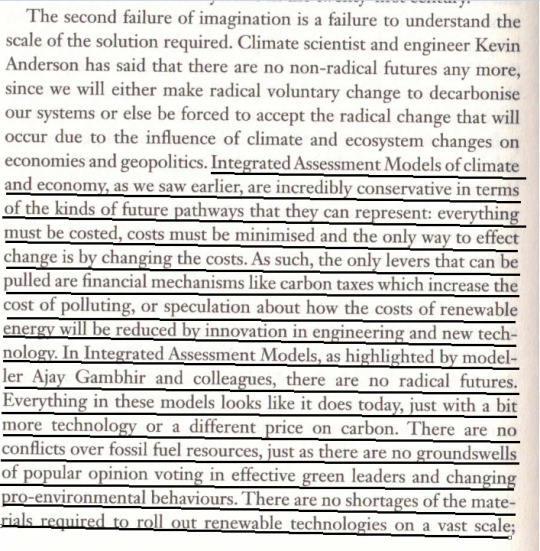
Octahedron(flatten) -> [Octahedron(flatten)](inflate)

Inflatable Octahedron
Another one of today's quick crafts is this "inflatable octahedron":
As I often have problems with having very limited storing space capacity I thought: "Why don't I make an inflatable model that can be stored in a flattened way? "
So, yeah... that is the result. 😅
- - -- ---
As for the crafting process: I used my beloved foldback-clamps (they are such multi-functional items! ) and some basic sticks... I fixated the vertices with basic masking tape...)
- - -- --- -----
some math fun facts:
An octahedron is a regular polyhedron (also called "platonic solid" ) and consists of
• 8 triangular faces
• 12 edges
• 6 vertices
#inflatable octahedron#octahedron#platonic solid#platonic solids#octahedra#geometry#math#mathematics#math art#math crafts#geometric models#geometric#artsy#crafting#crafty#diy#knottys crafts#flatten#mathy stuffy#math stuff
31 notes
·
View notes
Video
wiggle wiggle
#ace attorney#tgaa#dai gyakuten saiban#kazuma asougi#maybe i should have looked up actual mathematical models for waves with a node at one end#but can i really be bothered
355 notes
·
View notes
Text


6 notes
·
View notes
Text
haha what if I told you I'm working on...stuff..

ID: screenshot of a 3D model in Blender, it is a part of ray gun used by the killjoys. /End ID
#definitely do not have the computing power to make some killjoy figures like I'd want to try but a ray gun is a good substitute#it is little challenging to make it in blender especially since models in blender are divided into faces rather than being mathematical#shapes like they are in fusion but I do not have any measurements to do it in fusion so we'll see how this goes#(also ik the id is shit but idk how to describe guns tbh and well probably only few people will see it anyway)#danger days#killjoys#ttlotfk#ttlofk
30 notes
·
View notes
Text
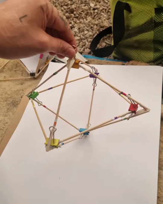
November 15th, 2023
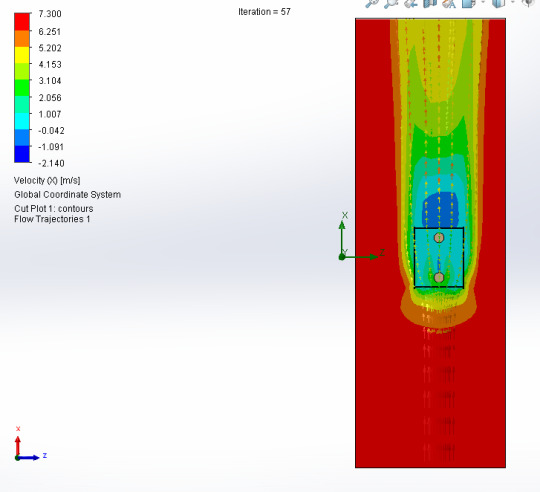
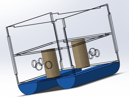
These photos are from the air flow simulation I did yesterday, to find out what impact the wind would have on the structure of the identification buoy. I recorded the animations to make it easier to analyze.
It was fun to do this, I discovered that I can make several different types of fluids, which could be useful in future projects.
The article is almost ready, along with the boat and buoy codes.
Here are the charts with results generated from Solidworks:

Generally I don't do this, but I'll put the translation of the analysis I put in the article here, maybe it can help someone.
Although it is not common to carry out engineering tests in this specific context, we chose to conduct an analysis dedicated to aerodynamic conditions, aiming to understand the effect of wind on the structural integrity of the buoy.
To carry out this study, we used Solidworks, making use of the fluid simulation system incorporated into the program.
Initially, we modeled the buoy structure, assigning specific materials to each component.
Subsequently, we establish the necessary boundary conditions to faithfully simulate the behavior of the structure in real conditions.
In the next step, we created surfaces that represent the wind pressure in the region where it impacts the buoy, and defined the area in which the wind pressure would be applied.
The application of wind loads and adjustment of analysis settings were carried out using the “Flow Simulation” tool.
This process allowed an accurate representation of the aerodynamic conditions on the buoy structure.
Additionally, we adjust relevant parameters for the analysis, ensuring a comprehensive approach.
The simulation execution culminated in the generation of a comprehensive report, documenting the results obtained. The interpretation of these results provided valuable insights into the structure's performance under simulated aerodynamic conditions.
This engineering test highlighted the importance of considering aerodynamic conditions when assessing structural integrity.
It is possible to highlight some fundamental reasons for the importance of this analysis, such as the assessment of structural integrity, assessment of operational safety, design optimization, which can result in savings in materials and manufacturing costs.
The Montagem_boia.SLDSAM model was configured with standard parameters, carrying out 57 iterations to achieve convergent results. The mesh was defined with basic dimensions (Nx = 40, Ny = 9, Nz = 17), and boundary conditions were established to represent the fluid environment of interest.
The physical time interval considered was 0 seconds, and the CPU time required for the simulation was also recorded.
The simulation results revealed an interesting distribution of fluid properties and flow characteristics. The total number of cells in the mesh was 7626, all occupied by the fluid. Among these, 1106 cells were in direct contact with solids.
The mesh dimensions (X,Y,Z) indicated a significant extension of the model, with minimum and maximum variations in each direction.
Analysis of the velocity field revealed a range of [0 m/s; 7,510 m/s], indicating different flow regimes within the simulation domain. The pressure varied between [101294.37 Pa; 101430.23 Pa], with a reference pressure of 101325.00 Pa. The temperature remained relatively constant, with values varying from [293.20 K; 293.21 K]. The fluid density showed a minimum variation, within the range of [1.20 kg/m^3; 1.21 kg/m^3].
There was no consideration of factors such as heat in solids, radiation, porous media and gravity to simplify the model to meet the specific objectives of this simulation.
Based on the analysis of the images obtained, the reduction in wind speed becomes visible when facing the structure of the identifying buoy.
Notably, the average wind speed in São Paulo, situated at 25km/h, is insufficient to cause damage to the aforementioned structure or to displace it from its original position.
It is also worth noting that, when encountering the obstacle represented by the buoy, the wind flow tends to bypass the structure mostly from above, to the detriment of the sides.
This observation suggests an effective resistance of the buoy to direct wind impact, contributing to its stability and structural robustness.
The results clearly indicate that the structure's resistance to wind action is remarkable, since the force exerted by the wind did not reach levels that would compromise the integrity or stability of the configuration.
The solidity of the structure in the face of these conditions suggests that the design presents a robust and adequate response to the expected wind loads.
Sorry for any grammatical errors ~
#stem#studyblr#stem academia#studyspo#study motivation#studyinspo#study aesthetic#engineering#studying#solidworks#3d model#computer engineering#mathematics#flow simulation#cad
17 notes
·
View notes
Text
I am desperate enough to ask this on f-ing tumblr, but nothing else has helped so far:
Does anyone know if the 2 equilibrium points (that are not (0,0,0)) of the Lorenz system are stable or not? And what is their classification (eg saddle point etc)?
I am going insane trying to figure it out but I just can't.
#lorenz system#lorenz butterfly#marhematical modelling#dynamical systems#mathematics#computational mathematics
12 notes
·
View notes
Last Seen Blogs

soundofnoise
Untitled


alhelo-m
Helos'

24-7sonlinepharmacy
24-7sonlinepharmacy

didyouknow-wp
Did you know?