randomdatablogger23

[randomdatablogger23]

K-Means Clustering

[randomdatablogger23]

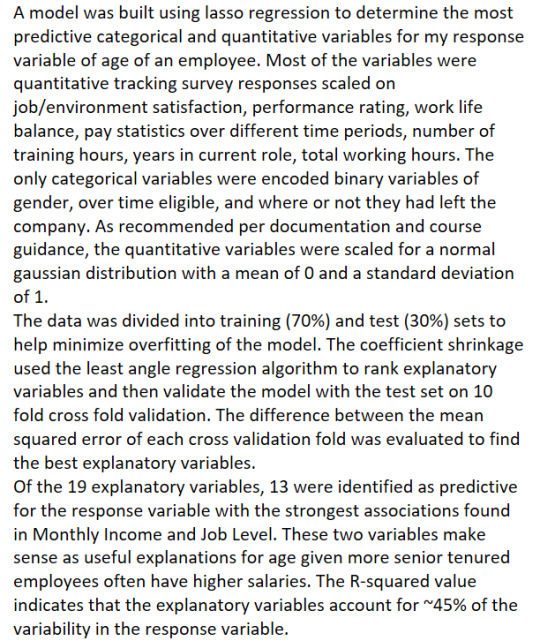
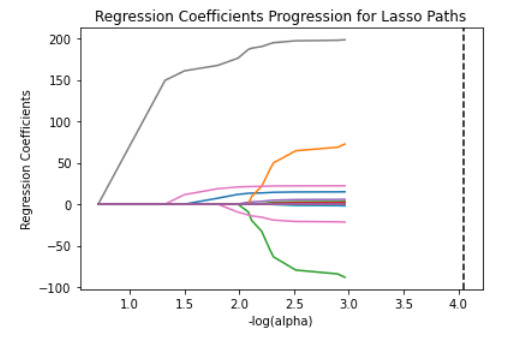
Lasso Regression Analysis

import pandas as pd import numpy as np import os import matplotlib.pylab as plt from sklearn.metrics import mean_squared_error from sklearn.model_selection import train_test_split from sklearn.linear_model import LassoLarsCV from sklearn import preprocessing

emp_data = pd.read_csv('IBM HR Attrition Data.csv')

emp_data['Age'].describe()

emp_data.isna().sum()

emp_data.dtypes

df = emp_data[['Age','Education','Gender','OverTime','Attrition',                       'HourlyRate','YearsInCurrentRole','DailyRate',               'DistanceFromHome','EmployeeCount','JobLevel','JobSatisfaction','EnvironmentSatisfaction',               'MonthlyRate','MonthlyIncome','NumCompaniesWorked','PerformanceRating',               'TotalWorkingYears','TrainingTimesLastYear','WorkLifeBalance','YearsInCurrentRole','TotalWorkingYears']] df['Attri'] = np.where(df['Attrition'].str.contains("Y"),1,0) df['Gender_cat'] = np.where(df['Gender'].str.contains("Female"),1,0) df['OT_cat'] = np.where(df['OverTime'].str.contains("Y"),1,0)

predict = df[['Education','Attri','MonthlyIncome','Gender_cat','OT_cat',                       'HourlyRate','YearsInCurrentRole','DailyRate',               'DistanceFromHome','EmployeeCount','JobLevel','JobSatisfaction','EnvironmentSatisfaction',               'MonthlyRate','PerformanceRating','NumCompaniesWorked',               'TotalWorkingYears','TrainingTimesLastYear','WorkLifeBalance','YearsInCurrentRole','TotalWorkingYears']] #'HourlyRate']]#,'Age','HourlyRate' predictors = predict.copy() predictors['Education'] = preprocessing.scale(predictors['Education']).astype('float64') predictors['Attri'] = preprocessing.scale(predictors['Attri']).astype('float64') predictors['MonthlyIncome'] = preprocessing.scale(predictors['MonthlyIncome']).astype('float64') predictors['Gender_cat'] = preprocessing.scale(predictors['Gender_cat']).astype('float64') predictors['OT_cat'] = preprocessing.scale(predictors['OT_cat']).astype('float64') predictors['HourlyRate'] = preprocessing.scale(predictors['HourlyRate']).astype('float64') predictors['YearsInCurrentRole'] = preprocessing.scale(predictors['YearsInCurrentRole']).astype('float64') predictors['DailyRate'] = preprocessing.scale(predictors['DailyRate']).astype('float64') predictors['DistanceFromHome'] = preprocessing.scale(predictors['DistanceFromHome']).astype('float64') predictors['EmployeeCount'] = preprocessing.scale(predictors['EmployeeCount']).astype('float64') predictors['JobLevel'] = preprocessing.scale(predictors['JobLevel']).astype('float64') predictors['JobSatisfaction'] = preprocessing.scale(predictors['JobSatisfaction']).astype('float64') predictors['EnvironmentSatisfaction'] = preprocessing.scale(predictors['EnvironmentSatisfaction']).astype('float64') predictors['MonthlyRate'] = preprocessing.scale(predictors['MonthlyRate']).astype('float64') predictors['PerformanceRating'] = preprocessing.scale(predictors['PerformanceRating']).astype('float64') predictors['NumCompaniesWorked'] = preprocessing.scale(predictors['NumCompaniesWorked']).astype('float64') predictors['TotalWorkingYears'] = preprocessing.scale(predictors['TotalWorkingYears']).astype('float64') predictors['TrainingTimesLastYear'] = preprocessing.scale(predictors['TrainingTimesLastYear']).astype('float64') predictors['WorkLifeBalance'] = preprocessing.scale(predictors['WorkLifeBalance']).astype('float64') predictors['YearsInCurrentRole'] = preprocessing.scale(predictors['YearsInCurrentRole']).astype('float64') predictors['TotalWorkingYears'] = preprocessing.scale(predictors['TotalWorkingYears']).astype('float64') targets = df.Age #MonthlyIncome predictors.head()

pred_train, pred_test, tar_train, tar_test = train_test_split(predictors, targets, test_size=.3) print(pred_train.shape,pred_test.shape,tar_train.shape,tar_test.shape)

model = LassoLarsCV(cv=10,precompute=False,max_iter=15).fit(pred_train,tar_train)

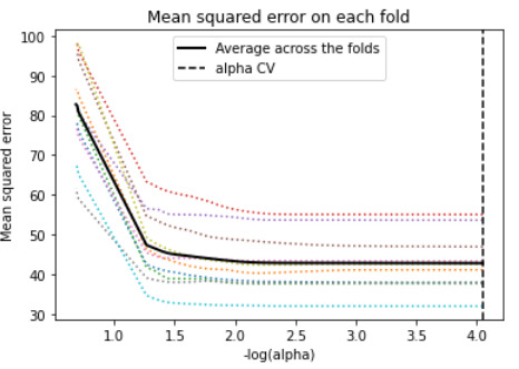
pred = dict(zip(predictors.columns,model.coef_)) df2 = pd.DataFrame(pred.values(),index=pred.keys(),columns=['coef']) df2['abs_coef'] = df2['coef'].apply(lambda x: abs(x)) df2.sort_values(by='abs_coef',ascending=False)

len(df2.index)

m_log_alphas = -np.log10(model.alphas_) ax = plt.gca() plt.plot(m_log_alphas, model.coef_path_.T) plt.axvline(-np.log10(model.alpha_), linestyle='--', color='k',            label='alpha CV') plt.ylabel('Regression Coefficients') plt.xlabel('-log(alpha)') plt.title('Regression Coefficients Progression for Lasso Paths')

m_log_alphascv = -np.log10(model.cv_alphas_) plt.figure() plt.plot(m_log_alphascv, model.mse_path_, ':') # plot mse with dotted line plt.plot(m_log_alphascv, model.mse_path_.mean(axis=-1), 'k',         label='Average across the folds', linewidth=2) plt.axvline(-np.log10(model.alpha_), linestyle='--', color='k',            label='alpha CV') plt.legend() plt.xlabel('-log(alpha)') plt.ylabel('Mean squared error') plt.title('Mean squared error on each fold')

train_error = mean_squared_error(tar_train, model.predict(pred_train)) test_error = mean_squared_error(tar_test, model.predict(pred_test)) print (f'training data MSE: {train_error}') print (f'test data MSE: {test_error}')

# R-square from training and test data rsquared_train = model.score(pred_train,tar_train) rsquared_test = model.score(pred_test,tar_test) print (f'training data R-square: {rsquared_train}') print (f'test data R-square: {rsquared_test}')

[randomdatablogger23]

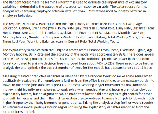
Random Forest Attrition Analysis

from pandas import Series, DataFrame import pandas as pd import numpy as np import os import matplotlib.pylab as plt from sklearn.model_selection import cross_validate from sklearn.model_selection import train_test_split #train_test_split from sklearn.tree import DecisionTreeClassifier from sklearn.metrics import classification_report import sklearn.metrics from sklearn import tree from sklearn import datasets from sklearn.ensemble import ExtraTreesClassifier from sklearn.ensemble import RandomForestClassifier

emp_data = pd.read_csv('IBM HR Attrition Data.csv')

emp_data.isna().sum()

emp_data.dtypes

emp_data['PerformanceRating'].describe()

df = emp_data[['Age','Education','Gender','OverTime',                       'HourlyRate','YearsInCurrentRole','DailyRate',               'DistanceFromHome','EmployeeCount','JobLevel','JobSatisfaction','EnvironmentSatisfaction',               'MonthlyRate','MonthlyIncome','NumCompaniesWorked','PerformanceRating',               'TotalWorkingYears','TrainingTimesLastYear','WorkLifeBalance','YearsInCurrentRole','TotalWorkingYears']] df['Gender_cat'] = np.where(df['Gender'].str.contains("Female"),1,0) df['OT_cat'] = np.where(df['OverTime'].str.contains("Y"),1,0)

predictors = df[['Age','Education','Gender_cat','OT_cat',                       'HourlyRate','YearsInCurrentRole','DailyRate',               'DistanceFromHome','EmployeeCount','JobLevel','JobSatisfaction','EnvironmentSatisfaction',               'MonthlyRate','MonthlyIncome','NumCompaniesWorked','PerformanceRating',               'TotalWorkingYears','TrainingTimesLastYear','WorkLifeBalance','YearsInCurrentRole','TotalWorkingYears']] #'HourlyRate']]#,'Age','HourlyRate' targets = emp_data.Attrition

pred_train, pred_test, tar_train, tar_test = train_test_split(predictors, targets, test_size=.4) print(pred_train.shape,pred_test.shape,tar_train.shape,tar_test.shape)

classifier = RandomForestClassifier(n_estimators=25) classifier = classifier.fit(pred_train,tar_train)

predictions = classifier.predict(pred_test) print(sklearn.metrics.confusion_matrix(tar_test,predictions)) sklearn.metrics.accuracy_score(tar_test,predictions)

model = ExtraTreesClassifier() model.fit(pred_train,tar_train) print(model.feature_importances_)

col_rank = {} for col,rk in zip(predictors.columns,model.feature_importances_):    col_rank[col] = rk

pred = pd.DataFrame(col_rank.values(),index=col_rank.keys(),columns={'rank'}) pred.head() pred.sort_values(by=['rank'],ascending=False)

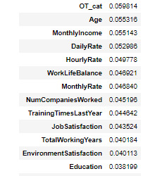
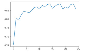
trees=range(25) accuracy=np.zeros(25)

for idx in range(len(trees)):    classifier = RandomForestClassifier(n_estimators=idx + 1)    classifier = classifier.fit(pred_train,tar_train)    predictions = classifier.predict(pred_test)    accuracy[idx] = sklearn.metrics.accuracy_score(tar_test, predictions)

plt.cla() plt.plot(trees, accuracy);

[randomdatablogger23]

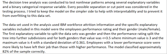
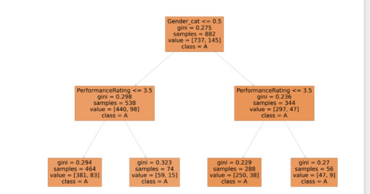
Decision Tree Modeling HR Attrition Data

from pandas import Series, DataFrame import pandas as pd import numpy as np import os import matplotlib.pylab as plt from sklearn.model_selection import cross_validate from sklearn.model_selection import train_test_split #train_test_split from sklearn.tree import DecisionTreeClassifier from sklearn.metrics import classification_report import sklearn.metrics from sklearn import tree

df.dtypes

emp_data = pd.read_csv('IBM HR Attrition Data.csv')

emp_data.isna().sum()

emp_data.dtypes

emp_data['PerformanceRating'].describe()

count    1470.000000 mean        3.153741 std         0.360824 min         3.000000 25%         3.000000 50%         3.000000 75%         3.000000 max         4.000000

df = emp_data[['Age','Education','Gender','OverTime',\                       'HourlyRate','YearsInCurrentRole','PerformanceRating',\                      'YearsInCurrentRole','TotalWorkingYears']] df['Gender_cat'] = np.where(df['Gender'].str.contains("Female"),1,0)

predictors = df[['PerformanceRating','Gender_cat']]  targets = emp_data.Attrition

pred_train, pred_test, tar_train, tar_test = train_test_split(predictors, targets, test_size=.4) print(pred_train.shape,pred_test.shape,tar_train.shape,tar_test.shape)

classifier = DecisionTreeClassifier() classifier = classifier.fit(pred_train,tar_train)

predictions = classifier.predict(pred_test) sklearn.metrics.confusion_matrix(tar_test,predictions) sklearn.metrics.accuracy_score(tar_test,predictions) 0.8163265306122449

fig = plt.figure(figsize=(75,50)) _ = tree.plot_tree(classifier,feature_names=predictors.columns,class_names='Attrition',filled=True)

[randomdatablogger23]

Logistic Regression in CBB Postseason

[randomdatablogger23]

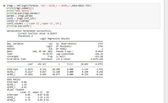
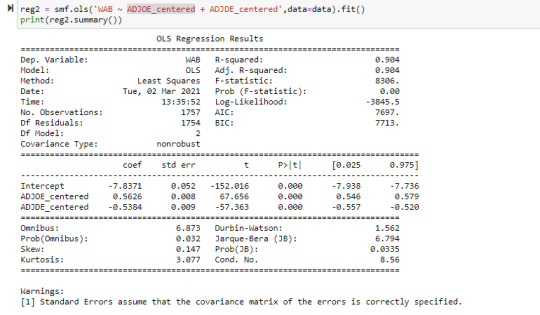
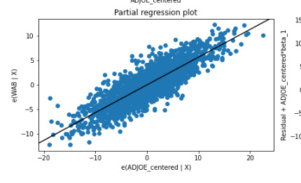
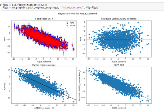
Multiple Linear Regression Relationship in College Basketball

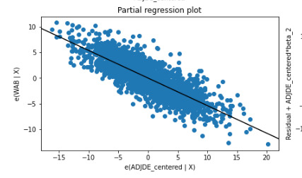
After incorporating two dependent variables into the regression model, it was evident that both were statistically significant in predicting wins metric (WAB: wins above bubble meaning the average team). Both adjusted offensive and defensive efficiency (after normalizing around 0) had a very low P-value (0.000) in the t-score. The offensive metric had a positive coefficient of 0.5626 as it has a positive linear relationship with the response variable and represents a half of a win more than the average team with each additional offensive efficiency. The defensive metric had a coefficient of -0.5384 as it had a negative relationship with the response variable and for each additional point decline in defensive efficiency there is just more than a half fewer wins. As hypothesized these two statistics reflect that they are significant in predicting wins during the college basketball tournament.

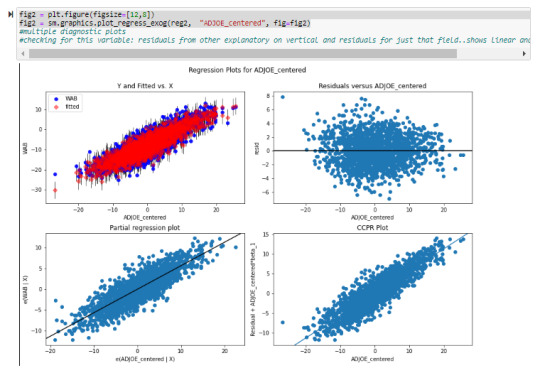
There was not evidence of confounding between these two variables as the P-values remained very statistically significant after adding in the additional explanatory variable (comparing against a linear model). Also from reviewing the partial regression plot the relationship between both adjusted offensive and defensive efficiency remained quite linear after accounting for the other variables.

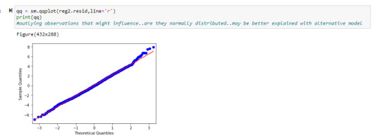
The QQ plot seems to indicate that there is a normal distribution as the points follow the sample quantile line fairly closely except for a few of the larger outliers.

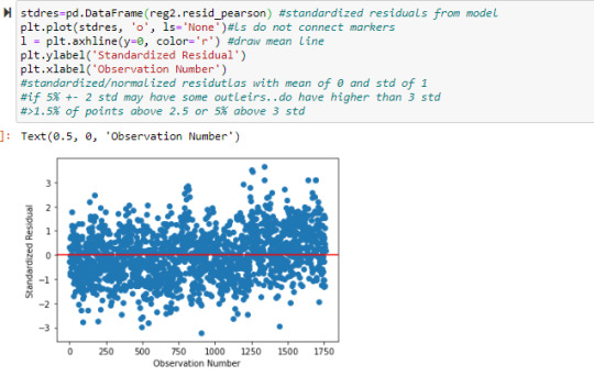
When reviewing the standardized residual plot the vast majority of points were still found within the 2 standard deviation cutoffs (34 teams >= 2 STD and 31 teams <=-2 STD) and those points including outliers only accounted for just under 4 percent of the data further indicating normalized variability.

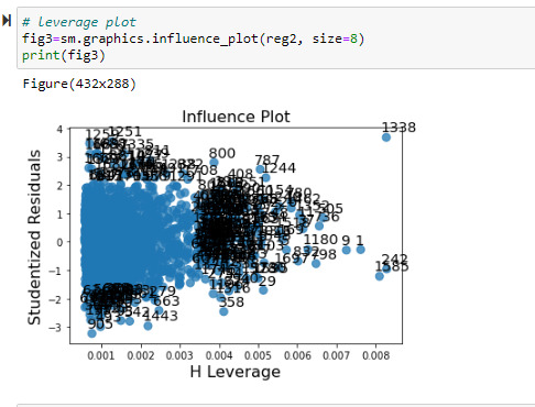
Despite the normal relationship the influence plot did indicate there were several outlier points, with the largest being point 1338, that had a large influence over the regression model. This is worth further consideration to exclude from the model to prevent undue influence in skewing some of the predicted values. Most of the influential points were in fact within 1 to 2 standard deviations from the mean.

Remaining code is included below:

[randomdatablogger23]

Testing the linear association between Adjusted Offensive Efficiency and Wins

There was a strong positive relationship between these two variables as shown in the below snapshot of code and visuals.

Framework import:

import numpy as np import pandas as pd import statsmodels.api as sm import statsmodels.formula.api as smf import matplotlib as plt import seaborn

pd.set_option("display.float_format",lambda x:'%.2f'%x)

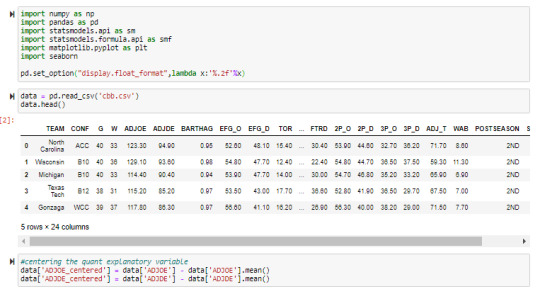
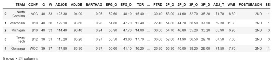
Previewing input data:

data = pd.read_csv('cbb.csv') data.head()

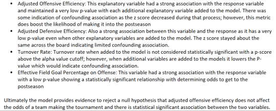
Scaling numerical explanatory variable around zero:

#centering the quant explanatory variable data['ADJOE_centered'] = data['ADJOE'] - data['ADJOE'].mean() data['ADJDE_centered'] = data['ADJDE'] - data['ADJDE'].mean()

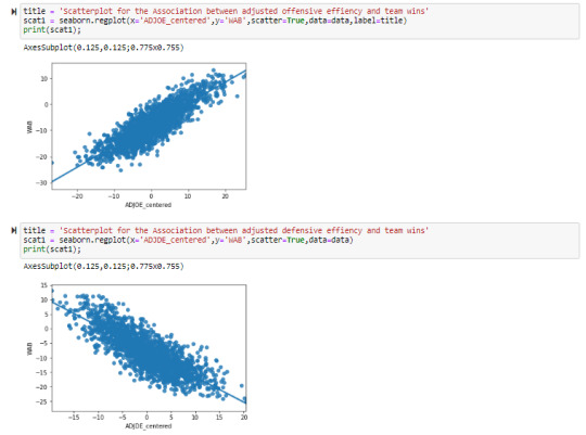
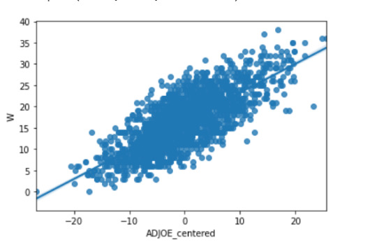
Building scatterplot of explanatory vs response:

title = 'Scatterplot for the Association between adjusted offensive effiency and team wins' scat1 = seaborn.regplot(x='ADJOE_centered',y='W',scatter=True,data=data,label=title) print(scat1);

Scatterplot for the association between adjusted offensive efficiency and team wins

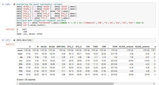
Running basic linear regression model:

print ("OLS regression model determining the association between offensive efficiency and win in Division 1 College Basketball") reg1 = smf.ols('W ~ ADJOE_centered', data=data).fit() #requests fit statistics print (reg1.summary()) # summary regression stats

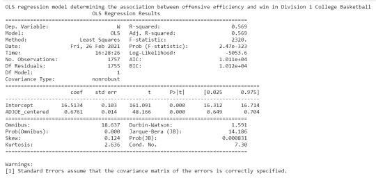
Summary:

The results from the simple linear regression model indicate that adjusted offensive efficiency is a statistically significant predictor for team wins as does the small P-value below the alpha level of 0.05. The scatterplot as well as the coefficient show a positive relationship between this set of explanatory and response variables. The R-squared statistic also indicates that approximately 56% of the variability in wins can be explained by the adjusted offensive efficiency.

[randomdatablogger23]

College Basketball Statistics Preliminary Write Up

Sample: The sample of data that I’ll be working through in the Regression Modeling course is a college basketball dataset showing team performance and postseason results in anticipation for March Madness. The data set includes results from 2015-2019 seasons for all 351 teams as well as the round in which they were eliminated if relevant from postseason data.

Procedures: The data was collected from Kaggle, a online data aggregator website owned by Google, which the individual poster scraped from another college basketball data website (https://barttorvik.com/). That website normally runs statistical analysis on some of advanced statistics for the sport and has built their own rating metric for teams.

Measures: There are a number of useful statistics that are captured in the dataset. Adjusted Offensive efficiency is an estimate of the number of points a team would score over 100 possessions, while adjusted defensive efficiency is the estimate of the number of points allowed to another team over 100 possessions. These two quantitative statistics are very useful to compare teams across conferences as they adjust for the level of competition that each team might play over the course of a season. The offensive efficiency ranges from 75 through 129, while defensive efficiency is from 84 through 125. Both variables will need to be scaled around 0 for reference to other potential explanatory variables. I will be comparing both of these variables individually to see if either is more predictive of the number of wins a team has over the course of a season.