
Last Seen Blogs

strictlycomedancing
Strictly Come Dancing

steampunk-subspace
STEAMSPACE'S BLOG!

leoclay8
Leo Clay 8

splicedm0th2
☆Timmy 2000☆

arichards00
anya.
Text
This week’s assignment involves running a k-means cluster analysis. Cluster analysis is an unsupervised machine learning method that partitions the observations in a data set into a smaller set of clusters where each observation belongs to only one cluster. The goal of cluster analysis is to group, or cluster, observations into subsets based on their similarity of responses on multiple variables. Clustering variables should be primarily quantitative variables, but binary variables may also be included.
Your assignment is to run a k-means cluster analysis to identify subgroups of observations in your data set that have similar patterns of response on a set of clustering variables.
Data
This is perhaps the best known database to be found in the pattern recognition literature. Fisher’s paper is a classic in the field and is referenced frequently to this day. (See Duda & Hart, for example.) The data set contains 3 classes of 50 instances each, where each class refers to a type of iris plant. One class is linearly separable from the other 2; the latter are NOT linearly separable from each other.
Predicted attribute: class of iris plant.
Attribute Information:
sepal length in cm
sepal width in cm
petal length in cm
petal width in cm
class
Iris Setosa
Iris Versicolour
Iris Virginica
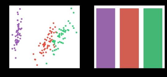
ResultsA k-means cluster analysis was conducted to identify classes of iris plants based on their similarity of responses on 4 variables that represent characteristics of the each plant bud. Clustering variables included 4 quantitative variables such as: sepal length, sepal width, petal length, and petal width.Data were randomly split into a training set that included 70% of the observations and a test set that included 30% of the observations. Then k-means cluster analyses was conducted on the training data specifying k=3 clusters (representing three classes: Iris Setosa, Iris Versicolour, Iris Virginica), using Euclidean distance.To describe the performance of a classifier and see what types of errors our classifier is making a confusion matrix was created. The accuracy score is 0.82, which is quite good due to the small number of observation (n=150)
0 notes
Text
This week’s assignment involves running a lasso regression analysis. Lasso regression analysis is a shrinkage and variable selection method for linear regression models. The goal of lasso regression is to obtain the subset of predictors that minimizes prediction error for a quantitative response variable. The lasso does this by imposing a constraint on the model parameters that causes regression coefficients for some variables to shrink toward zero. Variables with a regression coefficient equal to zero after the shrinkage process are excluded from the model. Variables with non-zero regression coefficients variables are most strongly associated with the response variable. Explanatory variables can be either quantitative, categorical or both.
Your assignment is to run a lasso regression analysis using k-fold cross validation to identify a subset of predictors from a larger pool of predictor variables that best predicts a quantitative response variable.
Data
Dataset description: hourly rental data spanning two years.
Dataset can be found at Kaggle
Features:
yr - year
mnth - month
season - 1 = spring, 2 = summer, 3 = fall, 4 = winter
holiday - whether the day is considered a holiday
workingday - whether the day is neither a weekend nor holiday
weathersit - 1: Clear, Few clouds, Partly cloudy, Partly cloudy
temp - temperature in Celsius
atemp - “feels like” temperature in Celsius
hum - relative humidity
windspeed (mph) - wind speed, miles per hour
windspeed (ms) - wind speed, metre per second
2: Mist + Cloudy, Mist + Broken clouds, Mist + Few clouds, Mist
3: Light Snow, Light Rain + Thunderstorm + Scattered clouds, Light Rain + Scattered clouds
4: Heavy Rain + Ice Pallets + Thunderstorm + Mist, Snow + Fog
Target:
cnt - number of total rentals esultsA lasso regression analysis was conducted to predict a number of total bikes rentals from a pool of 12 categorical and quantitative predictor variables that best predicted a quantitative response variable. Categorical predictors included weather condition and a series of 2 binary categorical variables for holiday and workingday to improve interpretability of the selected model with fewer predictors. Quantitative predictor variables include year, month, temperature, humidity and wind speed.Data were randomly split into a training set that included 70% of the observations and a test set that included 30% of the observations. The least angle regression algorithm with k=10 fold cross validation was used to estimate the lasso regression model in the training set, and the model was validated using the test set. The change in the cross validation average (mean) squared error at each step was used to identify the best subset of predictor variables.Of the 12 predictor variables, 10 were retained in the selected model:atemp: 63.56915200306693holiday: -282.431748735072hum: -12.815264427009353mnth: 0.0season: 381.77762475080044temp: 58.035647703871234weathersit: -514.6381162101678weekday: 69.84812053893549windspeed(mph): 0.0windspeed(ms): -95.71090321577515workingday: 36.15135752613271yr: 2091.5182927517903Train data R-square 0.7899877818517489
Test data R-square 0.8131871527614188During the estimation process, year and season were most strongly associated with the number of total bikes rentals, followed by temperature and weekday. Holiday, humidity, weather condition and wind speed (ms) were negative.
0 notes
Text
The second assignment deals with Random Forests. Random forests are predictive models that allow for a data driven exploration of many explanatory variables in predicting a response or target variable. Random forests provide importance scores for each explanatory variable and also allow you to evaluate any increases in correct classification with the growing of smaller and larger number of trees.
Run a Random Forest.
You will need to perform a random forest analysis to evaluate the importance of a series of explanatory variables in predicting a binary, categorical response variable.
Data
The dataset is related to red variants of the Portuguese “Vinho Verde” wine. Due to privacy and logistic issues, only physicochemical (inputs) and sensory (the output) variables are available (e.g. there is no data about grape types, wine brand, wine selling price, etc.).
The classes are ordered and not balanced (e.g. there are munch more normal wines than excellent or poor ones). Outlier detection algorithms could be used to detect the few excellent or poor wines. Also, we are not sure if all input variables are relevant. So it could be interesting to test feature selection methods.
Dataset can be found at UCI Machine Learning Repository
Attribute Information (For more information, read [Cortez et al., 2009]): Input variables (based on physicochemical tests):
1 - fixed acidity
2 - volatile acidity
3 - citric acid
4 - residual sugar
5 - chlorides
6 - free sulfur dioxide
7 - total sulfur dioxide
8 - density
9 - pH
10 - sulphates
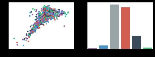
11 - alcoholOutput variable (based on sensory data):12 - quality (score between 0 and 10)ResultsRandom forest and ExtraTrees classifier were deployed to evaluate the importance of a series of explanatory variables in predicting a categorical response variable - red wine quality (score between 0 and 10). The following explanatory variables were included: fixed acidity, volatile acidity, citric acid, residual sugar, chlorides, free sulfur dioxide, total sulfur dioxide, density, pH, sulphates and alcohol.The explanatory variables with the highest importance score (evaluated by both classifiers) are alcohol, volatile acidity, sulphates. The accuracy of the Random forest and ExtraTrees clasifier is about 67%, which is quite good for highly unbalanced and hardly distinguished from each other classes. The subsequent growing of multiple trees rather than a single tree, adding a lot to the overall score of the model. For Random forest the number of estimators is 20, while for ExtraTrees classifier - 12, because the second classifier grows up much faster.
0 notes
Text
This week’s assignment involves decision trees, and more specifically, classification trees. Decision trees are predictive models that allow for a data driven exploration of nonlinear relationships and interactions among many explanatory variables in predicting a response or target variable. When the response variable is categorical (two levels), the model is a called a classification tree. Explanatory variables can be either quantitative, categorical or both. Decision trees create segmentations or subgroups in the data, by applying a series of simple rules or criteria over and over again which choose variable constellations that best predict the response (i.e. target) variable.
Run a Classification Tree.
You will need to perform a decision tree analysis to test nonlinear relationships among a series of explanatory variables and a binary, categorical response variable.
Data
Features are computed from a digitized image of a fine needle aspirate (FNA) of a breast mass [K. P. Bennett and O. L. Mangasarian: “Robust Linear Programming Discrimination of Two Linearly Inseparable Sets”, Optimization Methods and Software 1, 1992, 23-34].
Dataset can be found at UCI Machine Learn
In this Assignment the Decision tree has been applied to classification of breast cancer detection.
Attribute Information:
id - ID number
diagnosis (M = malignant, B = benign)
3-32 extra features
Ten real-valued features are computed for each cell nucleus:
a) radius (mean of distances from center to points on the perimeter)
b) texture (standard deviation of gray-scale values)
c) perimeter
d) area
e) smoothness (local variation in radius lengths)
f) compactness (perimeter^2 / area - 1.0)
g) concavity (severity of concave portions of the contour)
h) concave points (number of concave portions of the contour)
i) symmetry
j) fractal dimension (“coastline approximation” - 1)
All feature values are recoded with four significant digits.
Missing attribute values: none
Class distribution: 357 benign, 212 malignant

0 notes
Text
Logistic Regression Model
Preview
This assignment aims to examine the association of potential drug abuse/dependence prior to the last 12 months with major depression diagnosis in the last 12 months. among US adults aged from 18 to 30 years old (N=9535). All four explanatory variables were 4-level categorical and they were binned into 2 categories (0.=“No abuse/dependence, 1.=“Drug abuse/dependence”) for the purpose of these logistic models. More specifically, cannabis abuse/dependence (CANDEPPR12) is the primary explanatory variable and the potential confounding factors were cocaine (COCDEPPR12), heroine (HERDEPPR12) and alcohol (ALCDEPPR12). The response variable is major depression (MAJORDEP12) diagnosed in the last 12 months, which is categorical binary variable (0.=“No”, 1.=“Yes”). Therefore, we can evaluate if a specific drug abuse/dependence issue during the period prior to the last 12 months, is positively correlated with depression diagnosis in the last 12 months.
Results
The logistic regression model presented above illustrates the association of cannabis and cocaine abuse/dependence issue prior to the last 12 months with major depression, diagnosed in the last 12 months. The number of observations is 9535 (18-30) and the regression is significant at a P value of less than 0.0001 for cannabis and 0.001 for cocaine. The odds of having major depression were 2.5 times higher for participants with cannabis abuse/dependence than for participants without abuse/dependence (OR=2.59, 95% CI = 2.17-3.10, p=.0001). For cocaine the odds of having major depression were more than 1.7 times higher for individuals with cocaine abuse/dependence than for individuals without abuse/dependence (OR=1.73, 95% CI = 1.25-2.40, p=.001).
On the other hand, heroine’s relationship with major depression was not significant, with a p-value at 0.079 which is more than 0.05. Thus, the null hypothesis cannot be rejected.
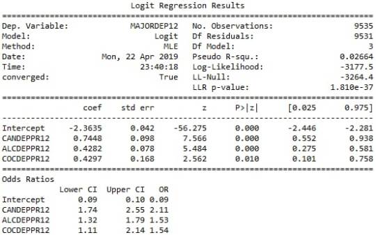
After adjusting for potential confounding factors alcohol and cocaine abuse/dependence, the odds of having depression were slightly more double for participants with cannabis issues than for participants without cannabis issues (OR=2.11, 95% CI = 1.74-2.55, p=.0001). Alcohol appeared to be also positively correlated with major depression, since alcoholic individuals had 1.5 times higher odds of getting diagnosed with this psychiatric disorder (OR=1.5, 95% CI = 1.32-1.79, p=.0001). Cocaine’s abuse/dependence odds seemed to be very close to alcohol (OR=1.54, 95% CI = 1.11-2.14, p=.01).
Summary
The logistic regression model revealed that cannabis, cocaine and alcohol were positively correlated with major depression, while heroine was not. Cannabis dependence was my primary explanatory variable and its significance appeared to remain steady when adding potential predictors (alcohol and cocaine) to the model. Therefore, there was no evidence of confounding for the association between my primary explanatory variable and the response variable. The results support my initial hypothesis.
0 notes
Text
Multiple Regression Model
Analysis
The multiple regression analysis aims to evaluate multiple predictors of the quantitative response variable, number of cannabis dependence symptoms (CanDepSymptoms). The primary explanatory variable is major depression diagnosis, in the last 12 months (MAJORDEP12), while the confounding factors are:
agebeganuse_c: Centered quantitative variable, which represents the age when individuals began using cannabis the most (values 5-64. Age).
numberjosmoked_c: Centered quantitative variable, which represents the number of joints smoked per day when using cannabis the most (values 1-98. Joints).
canuseduration_c: Centered quantitative variable, which represents the duration (in weeks) individuals used cannabis the most (values 1-2818. Weeks).
GENAXDX12: Categorical variable, which represents the diagnosis of general anxiety in the last 12 months (0.=“No”, 1.=“Yes”).
DYSDX12: Categorical variable, which represents the diagnosis of dysthymia in the last 12 months (0.=“No”, 1.=“Yes”).
SOCPDX12: Categorical variable, which represents the diagnosis of social phobia in the last 12 months (0.=“No”, 1.=“Yes”).
After adjusting the potential confounding factors, major depression (Beta=0.25, p=0.0001) was significantly and positively associated with number of cannabis dependence symptoms. The R-squared value was extremely small at 0.047 and F-statistic value is equal to 16.88. For the confounding variables:
Age when began using cannabis the most was not significantly associated with cannabis dependence symptoms and the null hypothesis cannot be rejected (Beta=-0.03, p=0.18).
Number of joints smoked per day was significantly associated with cannabis dependence symptoms, such that the larger quantity reported a greater number of cannabis dependence symptoms (Beta= 0.003, p=0.008).
Duration of cannabis use was not significantly associated with cannabis dependence symptoms and the null hypothesis cannot be rejected (Beta=9.4e-06, p=0.56).
General anxiety diagnosis was not significantly associated with cannabis dependence symptoms and the null hypothesis cannot be rejected (Beta=0.18, p=0.07).
Dysthymia diagnosis was significantly associated with cannabis dependence symptoms (Beta= 0.43, p=0.0001).
Social phobia diagnosis was significantly associated with cannabis dependence symptoms (Beta= 0.31, p=0.0001).
Report
To evaluate if the additional explanatory variables confounded the relationship between major depression diagnosis (primary explanatory variable) and cannabis dependence symptoms (response variable), I added the variables to my model one at a time. As a result, none of this variables confounded the association, since every time I added each predictor the p-value of major depression remained significant, at 0.0001. Therefore, the results of the multiple regression analysis for these adjusted potential confounding variables, supported my initial hypothesis.
Polynomial Regression
The second multiple regression analysis examines the association between the quantitative response variable, number of cannabis dependence symptoms (CanDepSymptoms) and the centered quantitative explanatory variable, number of joints smoked per day when using the most (numberjosmoked_c). A second order polynomial of number of joints variable (’numberjosmoked_c^2) was added to the regression equation in order to improve the fit of the model and capture the curve of linear relationship that was evident in the scatter plot. In addition, the recoded variable (CUFREQ) which represents the frequency of cannabis use (values 1-10, 1.=“Once a year”, 10.=“Every day”), was included to the model as a potential confounding factor. There is also a show that coefficients for the linear, and quadratic variables, remain significant after adjusting for frequency of cannabis use rate.
If we look at the results, it is noticeable that the value for the linear term for number of joints is 0.05, and the p value is less than 0.0001. In addition, the quadratic term is negative (-0.0006) and the p value is also significant (0.0001). The R square increases from 0.003 to 0.18., which means that adding the quadratic term for cannabis joints, increase the amount of variability in cannabis dependence symptoms that can be explained by cannabis use quantity from 0.3% to 18%. For the frequency of cannabis use the coefficient is equal to 0.09 and the p-value is significantly small, at 0.0001.
Diagnostic Plots
Q to Q Plot
This qq-plot evaluates the assumption that the residuals from our reggression model are normally distributed. A qq-plot, plots the quantiles of the residuals that we would theoretically see if the residuals followed a normal distribution, against the quantiles for the residuals estimated from the reggression model. It is noticeable that the residuals generally deviate from a straight line, especially at higher quantiles. This indicates that our residuals did not follow perfect normal distribution. This could mean that the curvilinear association that we observed in our scatter plot may not be fully estimated by the quadratic cannabis joints variable. Therefore, there might be other explanatory variables that could improve estimation of the observed curvilinearity.
Plot of standardized residuals for all observations
To evaluate the overall fit of the predicted values of the response variable to the observed values and to look for outliers, I created a plot for the standardized residuals of each observation. As we can see, most of the residuals fall between -2 and 2, but many of them fall also above 2. This indicates that we have several outliers, basically above the mean of 0. Furthermore, some of these outliers fall above 4 (extreme outliers) which suggests that the fit of the model is relatively poor and could be improved.
Regression plots for frequency of cannabis use
The plot in the upper right hand corner shows the residuals for each observation at different values of cannabis use frequency rate. There is clearly a funnel shaped pattern to the residuals where we can see that the absolute values of the them are small at lower values of frequency use rate, but then they start to get larger at higher levels. This indicates that this model does not predict cannabis dependence symptoms as well for individuals who have either high or low levels of cannabis use frequency rate. But is particularly worse predicting dependence symptoms for individuals with high frequency of cannabis use.
The partial regression residual plot, in the lower left hand corner, attempts to show the effect of adding cannabis use frequency rate as an additional explanatory variable to the model. For the frequency use rate variable, the values in the scatter plot are two sets of residuals. The residuals from a model predicting the cannabis dependence symptoms response from the other explanatory variables, excluding frequency of use, are plotted on the vertical access, and the residuals from the model predicting frequency of use from all the other explanatory variables are plotted on the horizontal access.What this means is that the partial regression plot shows the relationship between the response variable and specific explanatory variable, after controlling for the other explanatory variables. The residuals are spread out in a random pattern around the partial regression line and many of the residuals are pretty far from this line, indicating a great deal of cannabis dependence symptoms prediction error. Although cannabis use frequency rate shows a statistically significant association with cannabis dependence symptoms, this association is pretty weak after controlling for the number of joints smoked.
Leverage plot
The leverage plot attempts to identify observations that have an unusually large influence on the estimation of the predicted value of the response variable, cannabis dependence symptoms, or that are outliers, or both. We can see in the leverage plot is that we have a several outliers, contents that have residuals greater than 2 or less than -2. We’ve already identified some of these outliers in previous plots, but the plot also tells us which outliers have small or close to zero leverage values, meaning that although they are outlying observations, they do not have an undue influence on the estimation of the regression model.
0 notes
Text
Basic Linear Regression Model
Preview
The data was provided by the National Epidemiological Survey on Alcohol and Related Conditions (NESARC), which was conducted in a random sample of 43,093 U.S. adults and designed to determine the magnitude of alcohol use and psychiatric disorders. The data analytic subset, examined in this study, includes individuals aged between 18 and 30 years old who reported using cannabis at least once in their life (N=2,412). This assignment aims to evaluate the association between major depression diagnosis in the last 12 months (categorical explanatory variable) and cannabis dependence symptoms (quantitative response variable) during the same period, using a linear regression model.
Variables
Explanatory
Major depression diagnosis (MAJORDEP12) is a 2-level categorical variable (0=“No” , 1=“Yes”). The “No” category was initially coded “0”, thus there was no need for recode.
Frequency table of major depression diagnosis in cannabis users, ages 18-30
Response
Cannabis dependence symptoms (CanDepSymptoms) is a quantitative variable which I created for the purpose of the assignment. This variable was coded to represent the sum of 6 criteria:
Current cannabis abuse/dependence criteria, variables: S3CD5Q14C9 , S3CD5Q14C9
Longer period cannabis abuse/dependence criteria, variable: S3CD5Q14C3
Cannabis abuse/dependence sub-symptom criteria, which are:
Current cannabis use cut down criteria, variables: S3CD5Q14C2 , S3CD5Q14C1
Current reduce of important/pleasurable activities criteria, variables: S3CD5Q14C10 , S3CD5Q14C11
Current cannabis use continuation despite knowledge of physical or psychological problem criteria, variables: S3CD5Q14C13 , S3CD5Q14C12
Feel depressed because of cannabis effects wearing off, variable: S3CD5Q14C6C
Face sleeping difficulties because of cannabis effects wearing off, variable: S3CD5Q14C6R
Eat more because of cannabis effects wearing off, variable: S3CD5Q14C6H
Feel nervous or anxious because of cannabis effects wearing off, variable: S3CD5Q14C6I
Have fast heart beat because of cannabis effects wearing off, variable: S3CD5Q14C6D
Feel weak or tired because of cannabis effects wearing off, variable: S3CD5Q14C6B
Measures
I used ols function in order to estimate the regression equation and examine if major depression is correlated with cannabis dependence symptoms. Therefore, the F-statistic, P-value and parameter estimates (a.k.a. coefficients or beta weights) were calculated. In addition, the mean and the standard deviation were evaluated and the results were visualized with a bivariate bar graph.
Linear Regression Analysis Results
The linear regression model presented above aims to examine the association between major depression diagnosis in the last 12 months (categorical explanatory variable) and cannabis dependence symptoms (quantitative response variable), among U.S. adults aged between 18 and 30 years old. The number of observations that had valid data on both the response and explanatory variables and were therefore included in this analysis, was 2,412. The F-statistic is 60.34 and the P-value is 1.17e-14 (written in scientific notation). The P-value is considerably less than our alpha level of 0.05, which indicates that we can reject the null hypothesis and conclude that major depression diagnosis is significantly associated with cannabis dependence symptoms. In addition, the coefficient for major depression diagnosis is 0.38, and the intercept is 0.39. The P-value for our explanatory variable, in association with the response variable is p<0.0001 and the R-squared value, which is the proportion of the variance in cannabis dependence symptoms that can be explained by the major depression diagnosis, is significantly low at 2.4%.
Model Regression Equation
Bar Chart
The bivariate bar graph presented above illustrates the association between major depression, diagnosed in the last 12 months (explanatory variable) and cannabis dependence symptoms (response variable), in U.S. adults aged from 18 to 30 years old. The “No” category of major depression diagnosis is coded with “0” and the “Yes” is coded with “1”. As we can see, the individuals diagnosed with major depression in the last 12 months appeared to have marginally double cannabis dependence symptoms (mean = 0.77), compared to those who did not meet the criteria for this disorder (mean = 0.39). Therefore, major depression diagnosis is significantly associated with cannabis dependence symptoms.
0 notes
Text
Exploring Statistical Interactions
This assignment aims to statistically assess the evidence, provided by NESARC codebook, in favour of or against the association between cannabis use and major depression, in U.S. adults. More specifically, I examined the statistical interaction between frequency of cannabis use (10-level categorical explanatory, variable ”S3BD5Q2E”) and major depression diagnosis in the last 12 months (categorical response, variable ”MAJORDEP12”), moderated by variable “S1Q231“ (categorical), which indicates the total number of the people who lost a family member or a close friend in the last 12 months. This effect is characterised statistically as an interaction, which is a third variable that affects the direction and/or the strength of the relationship between the explanatory and the response variable and help us understand the moderation. Since I have a categorical explanatory variable (frequency of cannabis use) and a categorical response variable (major depression), I ran a Chi-square Test of Independence (crosstab function) to examine the patterns of the association between them (C->C), by directly measuring the chi-square value and the p-value. In addition, in order visualise graphically this association, I used factorplot function (seaborn library) to produce a bivariate graph. Furthermore, in order to determine which frequency groups are different from the others, I performed a post hoc test, using Bonferroni Adjustment approach, since my explanatory variable has more than 2 levels. In the case of ten groups, I actually need to conduct 45 pair wise comparisons, but in fact I examined indicatively two and compared their p-values with the Bonferroni adjusted p-value, which is calculated by dividing p=0.05 by 45. By this way it is possible to identify the situations where null hypothesis can be safely rejected without making an excessive type 1 error.
Regarding the third variable, I examined if the fact that a family member or a close friend died in the last 12 months, moderates the significant association between cannabis use frequency and major depression diagnosis. Put it another way, is frequency of cannabis use related to major depression for each level of the moderating variable (1=Yes and 2=No), that is for those whose a family member or a close friend died in the last 12 months and for those whose they did not? Therefore, I set new data frames (sub1 and sub2) that include either individuals who fell into each category (Yes or No) and ran a Chi-square Test of Independence for each subgroup separately, measuring both chi-square values and p-values. Finally, with factorplot function (seaborn library) I created two bivariate line graphs, one for each level of the moderating variable, in order to visualise the differences and the effect of the moderator upon the statistical relationship between frequency of cannabis use and major depression diagnosis. For the code and the output I used Spyder (IDE).
The moderating variable that I used for the statistical interaction is:
Output
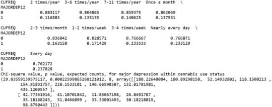
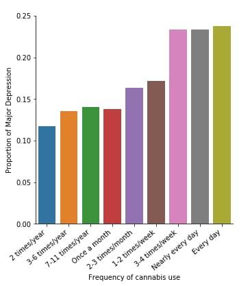
A Chi Square test of independence revealed that among cannabis users aged between 18 and 30 years old (subsetc1), the frequency of cannabis use (explanatory variable collapsed into 9 ordered categories) and past year depression diagnosis (response binary categorical variable) were significantly associated, X2 =29.83, 8 df, p=0.00022.

In the bivariate graph (C->C) presented above, we can see the correlation between frequency of cannabis use (explanatory variable) and major depression diagnosis in the past year (response variable). Obviously, we have a left-skewed distribution, which indicates that the more an individual (18-30) smoked cannabis, the better were the chances to have experienced depression in the last 12 months.
In the first place, for the moderating variable equal to 1, which is those whose a family member or a close friend died in the last 12 months (sub1), a Chi Square test of independence revealed that among cannabis users aged between 18 and 30 years old, the frequency of cannabis use (explanatory variable) and past year depression diagnosis (response variable) were not significantly associated, X2 =4.61, 9 df, p=0.86. As a result, since the chi-square value is quite small and the p-value is significantly large, we can assume that there is no statistical relationship between these two variables, when taking into account the subgroup of individuals who lost a family member or a close friend in the last 12 months.

Subsequently, for the moderating variable equal to 2, which is those whose a family member or a close friend did not die in the last 12 months (sub2), a Chi Square test of independence revealed that among cannabis users aged between 18 and 30 years old, the frequency of cannabis use (explanatory variable) and past year depression diagnosis (response variable) were significantly associated, X2 =37.02, 9 df, p=2.6e-05 (p-value is written in scientific notation). As a result, since the chi-square value is quite large and the p-value is significantly small, we can assume that there is a positive relationship between these two variables, when taking into account the subgroup of individuals who did not lose a family member or a close friend in the last 12 months.
In the bivariate line graph (C->C) presented above, we can see the correlation between frequency of cannabis use (explanatory variable) and major depression diagnosis in the past year (response variable), in the subgroup of individuals whose a family member or a close friend did not die in the last 12 months (sub2). Obviously, the direction of the distribution indicates a positive relationship between these two variables, which means that the frequency of cannabis use directly affects the proportions of major depression, regarding the individuals who did not experience a family/close death in the last 12 months.
Summary
It seems that both the direction and the size of the relationship between frequency of cannabis use and major depression diagnosis in the last 12 months, is heavily affected by a death of a family member or a close friend in the same period. In other words, when the incident of a family/close death is present, the correlation is considerably weak, whereas when it is absent, the correlation is significantly strong and positive. Thus, the third variable moderates the association between cannabis use frequency and major depression diagnosis.
0 notes
Text
Exploring Statistical Interactions
This assignment aims to statistically assess the evidence, provided by NESARC codebook, in favour of or against the association between cannabis use and major depression, in U.S. adults. More specifically, I examined the statistical interaction between frequency of cannabis use (10-level categorical explanatory, variable ”S3BD5Q2E”) and major depression diagnosis in the last 12 months (categorical response, variable ”MAJORDEP12”), moderated by variable “S1Q231“ (categorical), which indicates the total number of the people who lost a family member or a close friend in the last 12 months. This effect is characterised statistically as an interaction, which is a third variable that affects the direction and/or the strength of the relationship between the explanatory and the response variable and help us understand the moderation. Since I have a categorical explanatory variable (frequency of cannabis use) and a categorical response variable (major depression), I ran a Chi-square Test of Independence (crosstab function) to examine the patterns of the association between them (C->C), by directly measuring the chi-square value and the p-value. In addition, in order visualise graphically this association, I used factorplot function (seaborn library) to produce a bivariate graph. Furthermore, in order to determine which frequency groups are different from the others, I performed a post hoc test, using Bonferroni Adjustment approach, since my explanatory variable has more than 2 levels. In the case of ten groups, I actually need to conduct 45 pair wise comparisons, but in fact I examined indicatively two and compared their p-values with the Bonferroni adjusted p-value, which is calculated by dividing p=0.05 by 45. By this way it is possible to identify the situations where null hypothesis can be safely rejected without making an excessive type 1 error.
Regarding the third variable, I examined if the fact that a family member or a close friend died in the last 12 months, moderates the significant association between cannabis use frequency and major depression diagnosis. Put it another way, is frequency of cannabis use related to major depression for each level of the moderating variable (1=Yes and 2=No), that is for those whose a family member or a close friend died in the last 12 months and for those whose they did not? Therefore, I set new data frames (sub1 and sub2) that include either individuals who fell into each category (Yes or No) and ran a Chi-square Test of Independence for each subgroup separately, measuring both chi-square values and p-values. Finally, with factorplot function (seaborn library) I created two bivariate line graphs, one for each level of the moderating variable, in order to visualise the differences and the effect of the moderator upon the statistical relationship between frequency of cannabis use and major depression diagnosis. For the code and the output I used Spyder (IDE).

The moderating variable that I used for the statistical interaction is:
Output
A Chi Square test of independence revealed that among cannabis users aged between 18 and 30 years old (subsetc1), the frequency of cannabis use (explanatory variable collapsed into 9 ordered categories) and past year depression diagnosis (response binary categorical variable) were significantly associated, X2 =29.83, 8 df, p=0.00022.
In the bivariate graph (C->C) presented above, we can see the correlation between frequency of cannabis use (explanatory variable) and major depression diagnosis in the past year (response variable). Obviously, we have a left-skewed distribution, which indicates that the more an individual (18-30) smoked cannabis, the better were the chances to have experienced depression in the last 12 months.

In the first place, for the moderating variable equal to 1, which is those whose a family member or a close friend died in the last 12 months (sub1), a Chi Square test of independence revealed that among cannabis users aged between 18 and 30 years old, the frequency of cannabis use (explanatory variable) and past year depression diagnosis (response variable) were not significantly associated, X2 =4.61, 9 df, p=0.86. As a result, since the chi-square value is quite small and the p-value is significantly large, we can assume that there is no statistical relationship between these two variables, when taking into account the subgroup of individuals who lost a family member or a close friend in the last 12 months.
Subsequently, for the moderating variable equal to 2, which is those whose a family member or a close friend did not die in the last 12 months (sub2), a Chi Square test of independence revealed that among cannabis users aged between 18 and 30 years old, the frequency of cannabis use (explanatory variable) and past year depression diagnosis (response variable) were significantly associated, X2 =37.02, 9 df, p=2.6e-05 (p-value is written in scientific notation). As a result, since the chi-square value is quite large and the p-value is significantly small, we can assume that there is a positive relationship between these two variables, when taking into account the subgroup of individuals who did not lose a family member or a close friend in the last 12 months.
In the bivariate line graph (C->C) presented above, we can see the correlation between frequency of cannabis use (explanatory variable) and major depression diagnosis in the past year (response variable), in the subgroup of individuals whose a family member or a close friend did not die in the last 12 months (sub2). Obviously, the direction of the distribution indicates a positive relationship between these two variables, which means that the frequency of cannabis use directly affects the proportions of major depression, regarding the individuals who did not experience a family/close death in the last 12 months.
Summary
It seems that both the direction and the size of the relationship between frequency of cannabis use and major depression diagnosis in the last 12 months, is heavily affected by a death of a family member or a close friend in the same period. In other words, when the incident of a family/close death is present, the correlation is considerably weak, whereas when it is absent, the correlation is significantly strong and positive. Thus, the third variable moderates the association between cannabis use frequency and major depression diagnosis.
0 notes
Text
Hypothesis Testing and Pearson Correlation
This assignment aims to statistically assess the evidence, provided by NESARC codebook, in favor of or against the association between cannabis use and mental illnesses, such as major depression and general anxiety, in U.S. adults. More specifically, since my research question includes only categorical variables, I selected three new quantitative variables from the NESARC codebook. Therefore, I redefined my hypothesis and examined the correlation between the age when the individuals began using cannabis the most (quantitative explanatory, variable “S3BD5Q2F”) and the age when they experienced the first episode of major depression and general anxiety (quantitative response, variables “S4AQ6A” and ”S9Q6A”). As a result, in the first place, in order to visualize the association between cannabis use and both depression and anxiety episodes, I used seaborn library to produce a scatterplot for each disorder separately and interpreted the overall patterns, by describing the direction, as well as the form and the strength of the relationships. In addition, I ran Pearson correlation test (Q->Q) twice (once for each disorder) and measured the strength of the relationships between each pair of quantitative variables, by numerically generating both the correlation coefficients r and the associated p-values. For the code and the output I used Spyder (IDE).

The three quantitative variables that I used for my Pearson correlation tests are:
Output
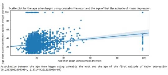
The scatterplot presented above, illustrates the correlation between the age when individuals began using cannabis the most (quantitative explanatory variable) and the age when they experienced the first episode of depression (quantitative response variable). The direction of the relationship is positive (increasing), which means that an increase in the age of cannabis use is associated with an increase in the age of the first depression episode. In addition, since the points are scattered about a line, the relationship is linear. Regarding the strength of the relationship, from the pearson correlation test we can see that the correlation coefficient is equal to 0.23, which indicates a weak linear relationship between the two quantitative variables. The associated p-value is equal to 2.27e-09 (p-value is written in scientific notation) and the fact that its is very small means that the relationship is statistically significant. As a result, the association between the age when began using cannabis the most and the age of the first depression episode is moderately weak, but it is highly unlikely that a relationship of this magnitude would be due to chance alone. Finally, by squaring the r, we can find the fraction of the variability of one variable that can be predicted by the other, which is fairly low at 0.05.
0 notes
Text
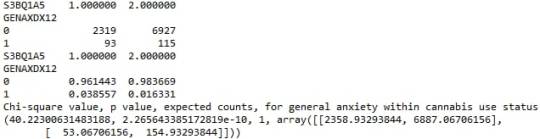
This assignment aims to directly test my hypothesis by evaluating, based on a sample of 2412 U.S. cannabis users aged between 18 and 30 years old (subsetc2), my research question with the goal of generalizing the results to the larger population of NESARC survey, from where the sample has been drawn. Therefore, I statistically assessed the evidence, provided by NESARC codebook, in favor of or against the association between cannabis use and mental illnesses, such as major depression and general anxiety, in U.S. adults. As a result, in the first place I used crosstab function, in order to produce a contingency table of observed counts and percentages for each disorder separately. Next, I wanted to examine if the cannabis use status (1=Yes or 2=No) variable ‘S3BQ1A5’, which is a 2-level categorical explanatory variable, is correlated with depression (‘MAJORDEP12’) and anxiety (‘GENAXDX12’) disorders, which are both categorical response variables. Thus, I ran Chi-square Test of Independence (C->C) twice and calculated the χ-squared values and the associated p-values for each disorder, so that null and alternate hypothesis are specified. In addition, in order visualize the association between frequency of cannabis use and depression diagnosis, I used factor plot function to produce a bivariate graph. Furthermore, I used crosstab function once again and tested the association between the frequency of cannabis use (‘S3BD5Q2E’), which is a 10-level categorical explanatory variable, and major depression diagnosis, which is a categorical response variable. In this case, for my third Chi-square Test of Independence (C->C), after measuring the χ-square value and the p-value, in order to determine which frequency groups are different from the others, I performed a post hoc test, using Bonferroni Adjustment approach, since my explanatory variable has more than 2 levels. In the case of ten groups, I actually need to conduct 45 pair wise comparisons, but in fact I examined indicatively two and compared their p-values with the Bonferroni adjusted p-value, which is calculated by dividing p=0.05 by 45. By this way it is possible to identify the situations where null hypothesis can be safely rejected without making an excessive type 1 error. For the code and the output I used Spyder (IDE).
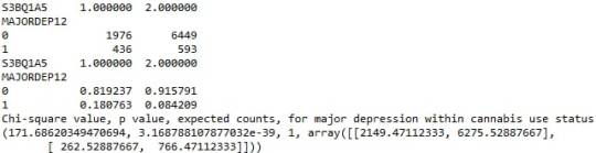
When examining the patterns of association between major depression (categorical response variable) and cannabis use status (categorical explanatory variable), a chi-square test of independence revealed that among young adults aged between 18 and 30 years old (subsetc1), those who were cannabis users, were more likely to have been diagnosed with major depression in the last 12 months (18%), compared to the non-users (8.4%), X2 =171.6, 1 df, p=3.16e-39 (p-value is written in scientific notation). As a result, since our p-value is extremely small, the data provides significant evidence against the null hypothesis. Thus, we reject the null hypothesis and accept the alternate hypothesis, which indicates that there is a positive correlation between cannabis use and depression diagnosis.
When examining the patterns of association between major depression (categorical response variable) and cannabis use status (categorical explanatory variable), a chi-square test of independence revealed that among young adults aged between 18 and 30 years old (subsetc1), those who were cannabis users, were more likely to have been diagnosed with major depression in the last 12 months (18%), compared to the non-users (8.4%), X2 =171.6, 1 df, p=3.16e-39 (p-value is written in scientific notation). As a result, since our p-value is extremely small, the data provides significant evidence against the null hypothesis. Thus, we reject the null hypothesis and accept the alternate hypothesis, which indicates that there is a positive correlation between cannabis use and depression diagnosis.
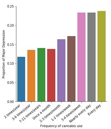
Similarly, the post hoc comparison (Bonferroni Adjustment) of rates of major depression by the pair of “Nearly every day” and “once a month” frequency categories, indicated that the p-value is 0.046 and the proportions of major depression diagnosis for each frequency group are 23.3% and 13.7% respectively. As a result, since the p-value is larger than the Bonferroni adjusted p-value (adj p-value = 0.05 / 45 = 0.0011<0.046), we can assume that these two rates are not significantly different from one another. Therefore, we accept the null hypothesis.
0 notes
Text
Hypothesis Testing and ANOVA
This assignment aims to directly test my hypothesis by evaluating, based on a sample of 2412 U.S. cannabis users aged between 18 and 30 years old (subsetc5), my research question with the goal of generalizing the results to the larger population of NESARC survey, from where the sample has been drawn. Therefore, I statistically assessed the evidence, provided by NESARC codebook, in favor of or against the association between cannabis use and mental illnesses, such as major depression and general anxiety, in U.S. adults. As a result, in the first place I used ols function in order to examine if depression (‘MAJORDEP12’) and anxiety (‘GENAXDX12’) disorders, which are both categorical explanatory variables, are correlated with the quantity of joints smoked per day when using the most ('S3BQ4’), which is a quantitative response variable. Thus, I ran ANOVA (Analysis Of Variance) method (C->Q) twice and calculated the F-statistics and the associated p-values for each disorder separately, so that null and alternate hypothesis are specified. Furthermore, I used ols function once again and tested the association between the frequency of cannabis use ('S3BD5Q2E’), which is a 10-level categorical explanatory variable, and the quantity of joints smoked per day when using the most ('S3BQ4’), which is a quantitative response variable. In this case, for my third one-way ANOVA (C->Q), after measuring the F-statistic and the p-value, I used Tukey HSDT to perform a post hoc test, that conducts post hoc paired comparisons in the context of my ANOVA, since my explanatory variable has more than 2 levels. By this way it is possible to identify the situations where null hypothesis can be safely rejected without making an excessive type 1 error. In addition, both means and standard deviations of joints quantity response variable, were measured separately in each ANOVA, grouped by the explanatory variables (depression, anxiety and frequency of cannabis use) using the group by function. For the code and the output I used Spyder (IDE).
Output
When examining the association between the number of joints smoked per day (quantitative response variable) and the past 12 months major depression diagnosis (categorical explanatory variable), an Analysis of Variance (ANOVA) revealed that among cannabis users aged between 18 and 30 years old (subsetc5), those diagnosed with major depression reported smoking slightly more joints per day (Mean=3.04, s.d. ±5.22) compared to those without major depression (Mean=2.39, s.d. ±4.16), F(1, 2368)=7.682, p=0.00562<0.05. As a result, since our p-value is extremely small, the data provides significant evidence against the null hypothesis. Thus, we reject the null hypothesis and accept the alternate hypothesis, which indicates that there is a positive correlation between depression diagnosis and quantity of joints smoked per day.
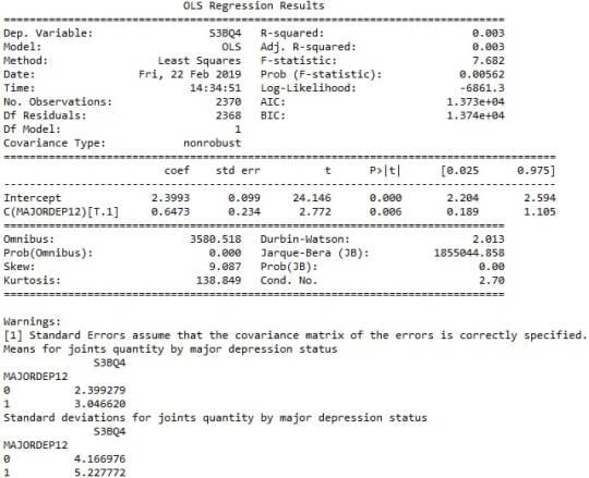
When testing the association between the number of joints smoked per day (quantitative response variable) and the past 12 months general anxiety diagnosis (categorical explanatory variable), an Analysis of Variance (ANOVA) revealed that among cannabis users aged between 18 and 30 years old (subsetc5), those diagnosed with general anxiety reported smoking marginally equal quantity of joints per day (Mean=2.68, s.d. ±3.15) compared to those without general anxiety (Mean=2.5, s.d. ±4.42), F(1, 2368)=0.1411, p=0.707>0.05. As a result, since our p-value is significantly large, in this case the data is not considered to be surprising enough when the null hypothesis is true. Consequently, there are not enough evidence to reject the null hypothesis and accept the alternate, thus there is no positive association between anxiety diagnosis and quantity of joints smoked per day.
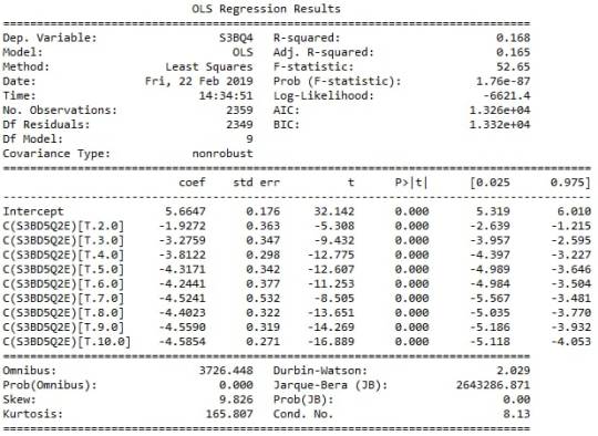
ANOVA revealed that among daily, cannabis users aged 18 to 30 years old (subsetc5), frequency of cannabis use (collapsed into 10 ordered categories, which is the categorical explanatory variable) and number of joints smoked per day (quantitative response variable) were relatively associated, F (9, 2349)=52.65, p=1.76e-87<0.05 (p value is written in scientific notation). Post hoc comparisons of mean number of joints smoked per day by pairs of cannabis use frequency categories, revealed that those individuals using cannabis every day (or nearly every day) reported smoking significantly more joints on average daily (every day: Mean=5.66, s.d. ±7.8, nearly every day: Mean=3.73, s.d. ±4.46) compared to those using 1 to 2 times per weak (Mean=1.85, s.d. ±1.81), or less. As a result, there are some pair cases in which using frequency and smoking quantity of cannabis, are positive correlated.
In order to conduct post hoc paired comparisons in the context of my ANOVA, examining the association between frequency of cannabis use and number of joints smoked per day when using the most, I used the Tukey HSD test. The table presented above, illustrates the differences in smoking quantity for each cannabis use frequency group and help us identify the comparisons in which we can reject the null hypothesis and accept the alternate, that is, in which reject equals true. In cases where reject equals false, rejecting the null hypothesis resulting in inflating a type 1 error.
0 notes
Text
Suicide Rates
Output with Frequency Tables at High Suicide Rate for Breast Cancer Rate, HIV Rate and Employment Rate Variables
Statistics for a Suicide Rate
count 191.000000
mean 9.640839
std 6.300178
min 0.201449
25% 4.988449
50% 8.262893
75% 12.328551
max 35.752872
Number of Breast Cancer Cases with a High Suicide Rate
# of Cases Freq. Percent Cum. Freq. Cum. Percent
6.51 6 11.32 6 11.32
15.14 14 26.42 20 37.74
23.68 5 9.43 25 47.17
32.22 7 13.21 32 60.38
40.76 2 3.77 34 64.15
49.30 4 7.55 38 71.70
57.84 5 9.43 43 81.13
66.38 1 1.89 44 83.02
74.92 3 5.66 47 88.68
83.46 4 7.55 51 96.23
NA 2 3.77 53 100.00
HIV Rate with a High Suicide Rate
Rate Freq. Percent Cum. Freq. Cum. Percent
0.03 39 73.58 6 11.32
2.64 4 7.55 20 37.74
5.23 2 3.77 25 47.17
7.81 0 0.00 32 60.38
10.40 0 0.00 34 64.15
12.98 2 3.77 38 71.70
15.56 1 1.89 43 81.13
18.15 0 0.00 44 83.02
20.73 0 0.00 47 88.68
23.32 1 1.89 51 96.23
NA 2 3.77 53 100.00
Employment Rate with a High Suicide Rate
Rate Freq. Percent Cum. Freq. Cum. Percent
37.35 2 3.77 6 11.32
41.98 2 3.77 20 37.74
46.56 7 13.21 25 47.17
51.14 8 15.09 32 60.38
55.72 16 30.19 34 64.15
60.30 4 7.55 38 71.70
64.88 5 9.43 43 81.13
69.46 2 3.77 44 83.02
74.04 3 5.66 47 88.68
78.62 3 5.66 51 96.23
NA 2 3.77 53 100.00
import pandas as pd
import numpy as np
# load gapminder dataset
data = pd.read_csv('gapminder.csv',low_memory=False)
# lower-case all DataFrame column names
data.columns = map(str.lower, data.columns)
# bug fix for display formats to avoid run time errors
pd.set_option('display.float_format', lambda x:'%f'%x)
# setting variables to be numeric
data['suicideper100th'] = data['suicideper100th'].convert_objects(convert_numeric=True)
data['breastcancerper100th'] = data['breastcancerper100th'].convert_objects(convert_numeric=True)
data['hivrate'] = data['hivrate'].convert_objects(convert_numeric=True)
data['employrate'] = data['employrate'].convert_objects(convert_numeric=True)
# display summary statistics about the data
print("Statistics for a Suicide Rate")
print(data['suicideper100th'].describe())
# subset data for a high suicide rate based on summary statistics
sub = data[(data['suicideper100th']>12)]
#make a copy of my new subsetted data
sub_copy = sub.copy()
# BREAST CANCER RATE
# frequency and percentage distritions for a number of breast cancer cases with a high suicide rate
#print('frequency for a number of breast cancer cases with a high suicide rate')
bc = sub_copy['breastcancerper100th'].value_counts(sort=False,bins=10)
#print(bc)
#print('percentage for a number of breast cancer cases with a high suicide rate')
pbc = sub_copy['breastcancerper100th'].value_counts(sort=False,bins=10,normalize=True)*100
#print(pbc)
# cumulative frequency and cumulative percentage for a number of breast cancer cases with a high suicide rate
bc1=[] # Cumulative Frequency
pbc1=[] # Cumulative Percentage
cf=0
cp=0
for freq in bc:
cf=cf+freq
bc1.append(cf)
pf=cf*100/len(sub_copy)
pbc1.append(pf)
#print('cumulative frequency for a number of breast cancer cases with a high suicide rate')
#print(bc1)
#print('cumulative percentage for a number of breast cancer cases with a high suicide rate')
#print(pbc1)
print('Number of Breast Cancer Cases with a High Suicide Rate')
fmt1 = '%s %7s %9s %12s %12s'
fmt2 = '%5.2f %10.d %10.2f %10.d %12.2f'
print(fmt1 % ('# of Cases','Freq.','Percent','Cum. Freq.','Cum. Percent'))
for i, (key, var1, var2, var3, var4) in enumerate(zip(bc.keys(),bc,pbc,bc1,pbc1)):
print(fmt2 % (key, var1, var2, var3, var4))
fmt3 = '%5s %10s %10s %10s %12s'
print(fmt3 % ('NA', '2', '3.77', '53', '100.00'))
# HIV RATE
# frequency and percentage distritions for HIV rate with a high suicide rate
#print('frequency for HIV rate with a high suicide rate')
hc = sub_copy['hivrate'].value_counts(sort=False,bins=7)
#print(hc)
#print('percentage for HIV rate with a high suicide rate')
phc = sub_copy['hivrate'].value_counts(sort=False,bins=7,normalize=True)*100
#print(phc)
# cumulative frequency and cumulative percentage for HIV rate with a high suicide rate
hc1=[] # Cumulative Frequency
phc1=[] # Cumulative Percentage
cf=0
cp=0
for freq in bc:
cf=cf+freq
hc1.append(cf)
pf=cf*100/len(sub_copy)
phc1.append(pf)
#print('cumulative frequency for HIV rate with a high suicide rate')
#print(hc1)
#print('cumulative percentage for HIV rate with a high suicide rate')
#print(phc1)
print('HIV Rate with a High Suicide Rate')
fmt1 = '%5s %12s %9s %12s %12s'
fmt2 = '%5.2f %10.d %10.2f %10.d %12.2f'
print(fmt1 % ('Rate','Freq.','Percent','Cum. Freq.','Cum. Percent'))
for i, (key, var1, var2, var3, var4) in enumerate(zip(hc.keys(),hc,phc,hc1,phc1)):
print(fmt2 % (key, var1, var2, var3, var4))
fmt3 = '%5s %10s %10s %10s %12s'
print(fmt3 % ('NA', '2', '3.77', '53', '100.00'))
# EMPLOYMENT RATE
# frequency and percentage distritions for employment rate with a high suicide rate
#print('frequency for employment rate with a high suicide rate')
ec = sub_copy['employrate'].value_counts(sort=False,bins=10)
#print(ec)
#print('percentage for employment rate with a high suicide rate')
pec = sub_copy['employrate'].value_counts(sort=False,bins=10,normalize=True)*100
#print(pec)
# cumulative frequency and cumulative percentage for employment rate with a high suicide rate
ec1=[] # Cumulative Frequency
pec1=[] # Cumulative Percentage
cf=0
cp=0
for freq in bc:
cf=cf+freq
ec1.append(cf)
pf=cf*100/len(sub_copy)
pec1.append(pf)
#print('cumulative frequency for employment rate with a high suicide rate')
#print(ec1)
#print('cumulative percentage for employment rate with a high suicide rate')
#print(pec1)
print('Employment Rate with a High Suicide Rate')
fmt1 = '%5s %12s %9s %12s %12s'
fmt2 = '%5.2f %10.d %10.2f %10.d %12.2f'
print(fmt1 % ('Rate','Freq.','Percent','Cum. Freq.','Cum. Percent'))
for i, (key, var1, var2, var3, var4) in enumerate(zip(ec.keys(),ec,pec,ec1,pec1)):
print(fmt2 % (key, var1, var2, var3, var4))
fmt3 = '%5s %10s %10s %10s %12s'
print(fmt3 % ('NA', '2', '3.77', '53', '100.00'))
0 notes
Text
Output
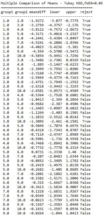
This graph is unimodal, with its highest pick at 0-20% of breast cancer rate. It seems to be skewed to the right as there are higher frequencies in lower categories than the higher categories.
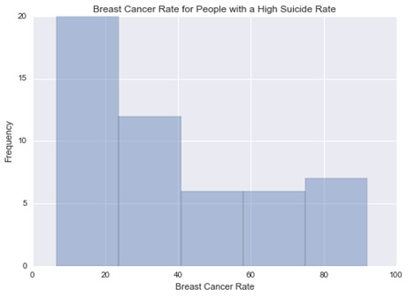
This graph is unimodal, with its highest pick at 0-1% of HIV rate. It seems to be skewed to the right as there are higher frequencies in lower categories than the higher categories.
This graph is unimodal, with its highest pick at the median of 55-60% employment rate. It seems to be a symmetric distribution as there are lower frequencies in lower and higher categories.
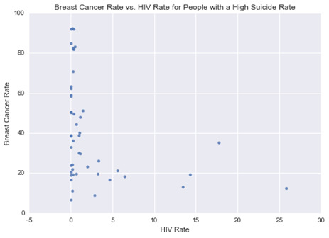
This graph plots the breast cancer rate vs. HIV rate for people with a high suicide rate. It shows that people with breast cancer are not infected with HIV.
Python Program
import pandas as pd
import numpy as np
import seaborn as sb
import matplotlib.pyplot as plt
# load gapminder dataset
data = pd.read_csv('gapminder.csv',low_memory=False)
# lower-case all DataFrame column names
data.columns = map(str.lower, data.columns)
# bug fix for display formats to avoid run time errors
pd.set_option('display.float_format', lambda x:'%f'%x)
# setting variables to be numeric
data['suicideper100th'] = data['suicideper100th'].convert_objects(convert_numeric=True)
data['breastcancerper100th'] = data['breastcancerper100th'].convert_objects(convert_numeric=True)
data['hivrate'] = data['hivrate'].convert_objects(convert_numeric=True)
data['employrate'] = data['employrate'].convert_objects(convert_numeric=True)
# display summary statistics about the data
# print("Statistics for a Suicide Rate")
# print(data['suicideper100th'].describe())
# subset data for a high suicide rate based on summary statistics
sub = data[(data['suicideper100th']>12)]
#make a copy of my new subsetted data
sub_copy = sub.copy()
# Univariate graph for breast cancer rate for people with a high suicide rate
plt.figure(1)
sb.distplot(sub_copy["breastcancerper100th"].dropna(),kde=False)
plt.xlabel('Breast Cancer Rate')
plt.ylabel('Frequency')
plt.title('Breast Cancer Rate for People with a High Suicide Rate')
# Univariate graph for hiv rate for people with a high suicide rate
plt.figure(2)
sb.distplot(sub_copy["hivrate"].dropna(),kde=False)
plt.xlabel('HIV Rate')
plt.ylabel('Frequency')
plt.title('HIV Rate for People with a High Suicide Rate')
# Univariate graph for employment rate for people with a high suicide rate
plt.figure(3)
sb.distplot(sub_copy["employrate"].dropna(),kde=False)
plt.xlabel('Employment Rate')
plt.ylabel('Frequency')
plt.title('Employment Rate for People with a High Suicide Rate')
# Bivariate graph for association of breast cancer rate with HIV rate for people with a high suicide rate
plt.figure(4)
sb.regplot(x="hivrate",y="breastcancerper100th",fit_reg=False,data=sub_copy)
plt.xlabel('HIV Rate')
plt.ylabel('Breast Cancer Rate')
plt.title('Breast Cancer Rate vs. HIV Rate for People with a High Suicide Rate')
# END
0 notes
Text
week 2 ass
Output with Frequency Tables at High Suicide Rate for Breast Cancer Rate, HIV Rate and Employment Rate Variables
Statistics for a Suicide Rate
count 191.000000
mean 9.640839
std 6.300178
min 0.201449
25% 4.988449
50% 8.262893
75% 12.328551
max 35.752872
Number of Breast Cancer Cases with a High Suicide Rate
# of Cases Freq. Percent Cum. Freq. Cum. Percent
6.51 6 11.32 6 11.32
15.14 14 26.42 20 37.74
23.68 5 9.43 25 47.17
32.22 7 13.21 32 60.38
40.76 2 3.77 34 64.15
49.30 4 7.55 38 71.70
57.84 5 9.43 43 81.13
66.38 1 1.89 44 83.02
74.92 3 5.66 47 88.68
83.46 4 7.55 51 96.23
NA 2 3.77 53 100.00
HIV Rate with a High Suicide Rate
Rate Freq. Percent Cum. Freq. Cum. Percent
0.03 39 73.58 6 11.32
2.64 4 7.55 20 37.74
5.23 2 3.77 25 47.17
7.81 0 0.00 32 60.38
10.40 0 0.00 34 64.15
12.98 2 3.77 38 71.70
15.56 1 1.89 43 81.13
18.15 0 0.00 44 83.02
20.73 0 0.00 47 88.68
23.32 1 1.89 51 96.23
NA 2 3.77 53 100.00
Employment Rate with a High Suicide Rate
Rate Freq. Percent Cum. Freq. Cum. Percent
37.35 2 3.77 6 11.32
41.98 2 3.77 20 37.74
46.56 7 13.21 25 47.17
51.14 8 15.09 32 60.38
55.72 16 30.19 34 64.15
60.30 4 7.55 38 71.70
64.88 5 9.43 43 81.13
69.46 2 3.77 44 83.02
74.04 3 5.66 47 88.68
78.62 3 5.66 51 96.23
NA 2 3.77 53 100.00
0 notes
Text
Changes in life expectancy in Russia in the mid-1990s
In this article, the authors state that the life expectancy in Russia has been changing due to the intricate pattern of trends in different causes of death, where some of which have their origins long in the past and others that results for contemporary circumstances. In the words of authors, the study provides further support for the view that alcohol has played an important part in the fluctuations in the life expectancy in Russia in the 1990s.
Drinking Pattern and Mortality:: The Italian Risk Factor and Life Expectancy Pooling Project
The purpose of this article is exactly to analyze the relationship between a particular aspect of drink pattern and a risk of all-cause and specific-cause mortality The results presented in this paper indicate that drinking patterns may have important health implications, impacting directly on the life expectancy.
Alcohol-related mortality by age and sex and its impact on life expectancy. Estimates based on the Finnish death register
This study was made in Finland and based on the “Finnish Death Register” that includes information on both the underlying and contributory causes of death and it yields an individual-level estimate of the contribution of alcohol to mortality. The data for 1987-1993 are used to examine alcohol-related mortality by cause of death. According to the results, 6% of all deaths were alcohol related. These deaths were responsible for a 2 year loss in life expectancy at age 15 years among men and 0.4 years among women.
alchohal consumption and life expentency
2 notes
·
View notes