cnamrata

[cnamrata]

Assignment 4: Data Management

To submit:

1. Create graphs of your variables one at a time (univariate graphs).Examine both their center and spread.

2. Create a graph showing the association between your explanatory and response variables (bivariate graph). Your output should be interpretable (i.e. organized and labeled).

Data set used: Gapminder dataset

Python Code:

--Start of Code--

import pandas import numpy import seaborn import matplotlib.pyplot as plt

data = pandas.read_csv('gapminder.csv', low_memory = False)

pandas.set_option('display.max_columns', None) pandas.set_option('display.max_rows', None)

pandas.set_option('display.float_format',lambda x: '%f' %x)

data["employrate"]= data["employrate"].convert_objects(convert_numeric=True) data["urbanrate"]= data["urbanrate"].convert_objects(convert_numeric=True) data["lifeexpectancy"]= data["lifeexpectancy"].convert_objects(convert_numeric=True) data["incomeperperson"]= data["incomeperperson"].convert_objects(convert_numeric=True) data["femaleemployrate"]= data["femaleemployrate"].convert_objects(convert_numeric=True) data["internetuserate"]= data["internetuserate"].convert_objects(convert_numeric=True)

#Univariate analysis of Employment Rate

sub1 = data[ (data['employrate']>=50) & (data['employrate']<=100) & (data['urbanrate']>= 40)]

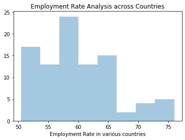
#copies sub1 data into a new subset called sub2 sub2 = sub1.copy() dist1=seaborn.distplot(sub2['employrate'].dropna(),kde=False); plt.xlabel('Employment Rate in various countries') plt.title('Employment Rate Analysis across Countries')

desc1=data['employrate'].describe()

print(desc1)

desc2=data['urbanrate'].describe()

print(desc2)

desc3=data['internetuserate'].describe()

print(desc3)

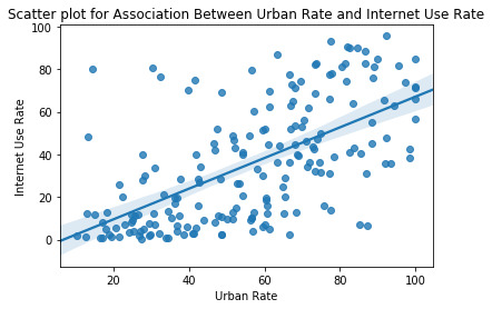
#Bivariate analysis of internet user rate, life expectancy etc. scat1=seaborn.regplot(x="urbanrate",y="internetuserate", data=data) plt.xlabel('Urban Rate') plt.ylabel('Internet Use Rate') plt.title('Scatter plot for Association Between Urban Rate and Internet Use Rate')

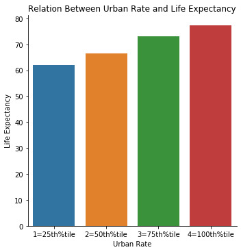
print('Urban Rate in 4 Quartiles') data['UrbanQuartile']=pandas.qcut(data.urbanrate, 4, labels=["1=25th%tile","2=50th%tile","3=75th%tile","4=100th%tile"]) c1 = data['UrbanQuartile'].value_counts(sort=False, dropna=True) print(c1) fact1=seaborn.factorplot(x='UrbanQuartile', y='lifeexpectancy', data=data, kind="bar", ci=None)

plt.xlabel('Urban Rate') plt.ylabel('Life Expectancy') plt.title('Relation Between Urban Rate and Life Expectancy')

c2= data.groupby('UrbanQuartile').size() print(c2)

--End of code--

Output:

count   178.000000 mean     58.635955 std      10.519455 min      32.000000 25%      51.225000 50%      58.700000 75%      64.975000 max      83.200000 Name: employrate, dtype: float64

count   203.000000 mean     56.769360 std      23.844933 min      10.400000 25%      36.830000 50%      57.940000 75%      74.210000 max     100.000000 Name: urbanrate, dtype: float64

count   192.000000 mean     35.632760 std      27.780433 min       0.210000 25%      10.000000 50%      31.810000 75%      56.415000 max      95.640000 Name: internetuserate, dtype: float64

Urban Rate in 4 Quartiles 1=25th%tile     51 2=50th%tile     51 3=75th%tile     50 4=100th%tile    51

Description of Output:

- The output of desc function gives frequency, count, spread of the variables employment rate, urban rate and internet use rate of various countries.

From the output of employment rate, we can see that the average employment rate among the given set of countries is 58.6% and the standard deviation is 10.5% indicating that most of the values are concentrated around the mean.

The spread of employment rate is given as maximum-minimum which is 51.2%

- I did univariate analysis on Employment rate by country by using a histogram. Based on the analysis, we can conclude that about highest number of countries (~24) are found to have employment rate of around 57%. Number of countries with highest employment rate (~75%) is 5.

- I used the Scatter Plot function to analyse the association of urban rate (independent variable) and internet usage rate (dependent variable). From the plot, we can conclude that internet usage rate increases linearly as urban rate increases. However, the plot also indicates that the data is not concentrated along the line of best fit but is scattered. 

- I did a bivariate analysis to arrive at the relation of urban rate and life expectancy. Urban Rate is divided into 4 quartiles. It can be concluded that with increase in urban rate, life expectancy rate also increases.

[cnamrata]

Assignment 3- Making Data Management Decisions

To submit:  Write a successful program that manages your data, create a blog entry where you post your program and the results/output that displays at least 3 of your data managed variables as frequency distributions. Write a few sentences describing these frequency distributions in terms of the values the variables take, how often they take them, the presence of missing data, etc.

I have used the gapminder data set to display the frequency distribution of variables such as employrate and life expectancy rate given a level of urban rate and alcohol consumption respectively.

Python Program for frequency distribution:

Below is the program for frequency distribution in Python:

--Start of program--

import pandas import numpy

data = pandas.read_csv('gapminder.csv', low_memory = False) pandas.set_option('display.float_format',lambda x: '%f' %x)

print("Returns the count of number of countries in each employment level") c1=data.groupby("Countrylevelofemployment").size() print (c1)

print("Returns % distribution of countries in each employment level") p1=data.groupby("Countrylevelofemployment").size() * 100/len(data) print(p1)

data["employrate"]= data["employrate"].convert_objects(convert_numeric=True) data["urbanrate"]= data["urbanrate"].convert_objects(convert_numeric=True) data["lifeexpectancy"]= data["lifeexpectancy"].convert_objects(convert_numeric=True) data["alcconsumption"]= data["alcconsumption"].convert_objects(convert_numeric=True)

sub1 = data[ (data['employrate']>=50) & (data['employrate']<=100) & (data['urbanrate']>= 40)] sub3=data[ (data['lifeexpectancy']>=60) & (data['alcconsumption']>0.5)]

sub2 = sub1.copy() sub4 = sub3.copy()

print('Quartile distribution of countries based on employment rate given a level of urban rate') sub2 ['Employrate 4']=pandas.qcut(sub2.employrate,4,labels=["1-25%tile","2-50%tile","3-75%tile","4-100%tile"]) c2=sub2['Employrate 4'].value_counts(sort=False,dropna=True) print(c2)

print('Quartile distribution of countries based on life expectancy given a level of alcohol consumption') sub4 ['Life expectancy 4']=pandas.qcut(sub4.lifeexpectancy,4,labels=["1-25%tile","2-50%tile","3-75%tile","4-100%tile"]) c3=sub4['Life expectancy 4'].value_counts(sort=False,dropna=True) print(c3)

-- End of Program--

Output of the program:

Returns the count of number of countries in each employment level Countrylevelofemployment Average Employment Rate (50% to 70%)    114 Data Not Available                       35 High Employment Rate (> 70%)             27 Low Employment Rate (0% to 50%)          37 dtype: int64 Returns % distribution of countries in each employment level Countrylevelofemployment Average Employment Rate (50% to 70%)   53.521127 Data Not Available                     16.431925 High Employment Rate (> 70%)           12.676056 Low Employment Rate (0% to 50%)        17.370892 dtype: float64 Quartile distribution of countries based on employment rate given a level of urban rate 1-25%tile     25 2-50%tile     23 3-75%tile     22 4-100%tile    23 Name: Employrate 4, dtype: int64 Quartile distribution of countries based on life expectancy given a level of alcohol consumption 1-25%tile     33 2-50%tile     32 3-75%tile     32 4-100%tile    32 Name: Life expectancy 4, dtype: int64

Description of the program:

The program gives:

a) The distribution of countries based on level of employees and % level of employment in each level. This clearly specifies blank rows where data is not available

b) Quartile distribution of countries where employment rate is between 50% to 100% and where urban rate is greater than 40%. As per the output, we can see that the distribution of countries is almost equal across the quartiles. The output excludes countries/rows where data is not available.

c) Quartile distribution of countries where life expectancy is greater than 60% and alcohol consumption is greater than 0.5. As per the output, we can see that the distribution of countries is almost equal across the quartiles. The output excludes countries/rows where data is not available.

[cnamrata]

Assignment 2: Data Management and Visualization

Requirement of Assignment 2: Following completion of your first program, create a blog entry where you post 1) your program 2) the output that displays three of your variables as frequency tables and 3) a few sentences describing your frequency distributions in terms of the values the variables take, how often they take them, the presence of missing data, etc.

1. Python program

I ran the program in python and below is the code:

import pandas import numpy

data = pandas.read_csv('gapminder.csv', low_memory = False)

print("Returns the count of number of countries in each employment level") c1=data.groupby("Countrylevelofemployment").size() print (c1)

print("Returns % distribution of countries in each employment level") p1=data.groupby("Countrylevelofemployment").size() * 100/len(data) print(p1)

print("Returns the count of countries falling under various income levels") c2=data.groupby("Incomelevel").size() print(c2)

print ("Returns % of countries falling in each income level") p2=data.groupby("Incomelevel").size()*100/len(data) print (p2)

print("Returns internet usage level across countries") c3=data.groupby("Internetusagelevel").size() print(c3)

print("Returns % countries in each internet usage bracket") p3=data.groupby("Internetusagelevel").size() *100/len(data) print(p3)

print("Returns the number of countries at each level of urbanization") c4=data.groupby("Urbanizationlevel").size() print(c4)

print("Returns % of countries at each level of urbanization") p4=data.groupby("Urbanizationlevel").size()*100/len(data) print(p4)

2. Output of the program

Returns the count of number of countries in each employment level Countrylevelofemployment Average Employment Rate (50% to 70%)    114 Data Not Available                       35 High Employment Rate (> 70%)             27 Low Employment Rate (0% to 50%)          37 dtype: int64

Returns % distribution of countries in each employment level Countrylevelofemployment Average Employment Rate (50% to 70%)   53.521127 Data Not Available                     16.431925 High Employment Rate (> 70%)           12.676056 Low Employment Rate (0% to 50%)        17.370892 dtype: float64

Returns the count of countries falling under various income levels Incomelevel Data Not Available                                  23 High income countries (> $30,000)                   16 Low income countries ($0 to $10000)                143 Mid level income countries ($10,000 to $30,000)     31 dtype: int64

Returns % of countries falling in each income level Incomelevel Data Not Available                                10.798122 High income countries (> $30,000)                  7.511737 Low income countries ($0 to $10000)               67.136150 Mid level income countries ($10,000 to $30,000)   14.553991 dtype: float64

Returns internet usage level across countries Internetusagelevel Data Not Available                    21 High internet usage (> 60%)           47 Low internet usage (0% to 30%)        93 Medium internet usage (30% to 60%)    52 dtype: int64

Returns % countries in each internet usage bracket Internetusagelevel Data Not Available                    9.859155 High internet usage (> 60%)          22.065728 Low internet usage (0% to 30%)       43.661972 Medium internet usage (30% to 60%)   24.413146 dtype: float64

Returns the number of countries at each level of urbanization Urbanizationlevel Data Not Available            10 Developed (> 70%)             64 Developing (40% to 70%)       80 Underdeveloped (0% to 40%)    59 dtype: int64

Returns % of countries at each level of urbanization Urbanizationlevel Data Not Available            4.694836 Developed (> 70%)            30.046948 Developing (40% to 70%)      37.558685 Underdeveloped (0% to 40%)   27.699531 dtype: float64

3. Description of the program

I chose GapMinder dataset in which the entire data is not absolute numbers. Data is either in percentages such as the variable ‘employrate’ which was  % of people employed in the entire population of the country or variables like ‘income per person’ which describe the income earned on a per capita basis. Frequency distribution on such data would not have given relevant results. Hence, I introduced few dummy variables which i used for frequency distribution. They are as follows:

A) Countrylevelofemployment: This variable takes 4 values namely

Low Employment Rate for countries whose employment rate is between 0 to 50%

Average Employment Rate for countries whose employment rate is between 50 to 70% and 

High Employment Rate for countries whose employment rate is greater than 70%

Data Not Available for countries which have no information available

B) Incomelevel: This variable takes 4 values namely

Low income countries for those countries whose per capita income level is less than $10K

Mid level income countries for those countries whose per capita income is between $10K to $30K

High income countries for those countries whose per capita income is greater than $30K

and Data Not Available incase no information was available about that country

C) Internetusagelevel: This variable takes 4 values namely

Low internet usage for countries whose rate is less than 30%

Medium internet usage for countries whose usage rate is between 30 to 60% 

High internet usage for countries whose usage rate is greater than 60% and

Data Not Available for countries on which information was available

D) Urbanization level: This variable takes 4 value namely

Under developed for countries whose urbanization levels were less than 40%

Developing countries were the ones with urbanization rate between 40 to 70%

Developed countries were the ones with urbanization rate greater than 70% and

Data Not Available for those countries which had no information available

Observation from program output:

Based on the output of the program, highest values across each distribution are given below

i) 53.5% of the countries fall under Average Employment Rate (50% to 70%)

ii) 67.1% of countries are low income countries (percapita income of $0 to $10,000)

iii) 43.7% of countries had low internet usage (0% to 30%)

iv) 37.6% of countries were developing (40% to 70%). This is closely followed by 30% of countries which were developed (>70% urbanization rate) which is in turn closely followed by 27.7% of countries whch were under developed (<40% urbanization rate). 

[cnamrata]

Assignment 1 for Data Management and Visualization

Selecion of dataset- Gap minder dataset

I would like to select female employment as my research area with the following being my primary research questions:

a) Is female employment rate dependent on total employment rate?

b) Does income per person of a country influence employment of females in that country?

c) Does female employment rate depend on internet use rate in a country?

d) Is urbanization of a country a good indicator of female employment?

Hypothesis- Female employment rate depends on total employment rate of the country, income per person, internet usage and urban rate

Variables to be used: 

femaleemployrate

internetuserrate

employrate

income per person

urbanrate

Secondary research question:

Is life expectancy of a country dependent on female employment rate?

Hypothesis- Life expectancy in a country is dependent on female employment rate

Variables to be used: 

femaleemployrate

lifeexpectancy

References:

1. Understanding income inequalities in health among men and women in Britain and Finland

Ossi Rahkonen, Sara Arber, Eero Lahelma, Pekka Martikainen, Karri Silventoinen

International Journal of Health Services 30 (1), 27-47, 2000

2.The changing status of women in India

R.N. Ghosh, K.C. Roy 

International Journal of Social Economics

ISSN: 0306-8293