excelunlocked-blog - Tumblr blog

excelunlocked-blog · 4 years

Text

Amazing Feature in Excel - Custom List in Excel

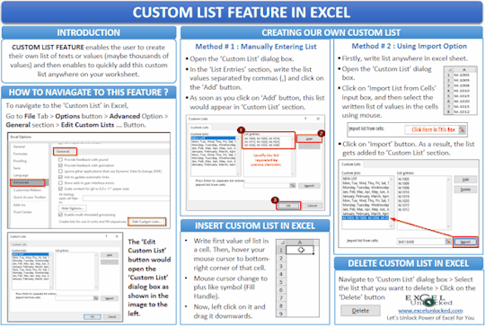
In this blog, we would learn what is a custom list in Excel and how to create a new custom list. We would also learn to sort the data based on a custom list in Excel. The Custom List feature in Excel is a life-saver tool provided by Microsoft in Excel utility, which can save a lot of your time and precious efforts.

What are Custom Lists in Excel

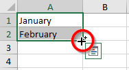
A Custom list feature is an in-built feature provided by excel that enables the user to create their own list of texts or values (maybe thousands of values) and then enables to quickly add this custom list anywhere on your worksheet by simply selecting the list or by dragging it. Before, starting to learn to add a custom list, let us do one small activity. Firstly, write the month name ‘January’ in any of the cells in Excel and then, in the cell just below it, write the month ‘February’. Now, select these cells and hover your mouse cursor to the bottom right corner of the selected range, till the cursor changes to the plus like symbol (called as Fill Handle)

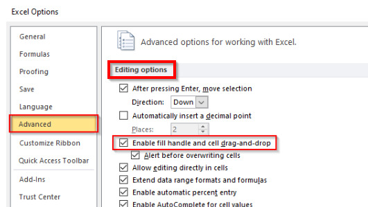
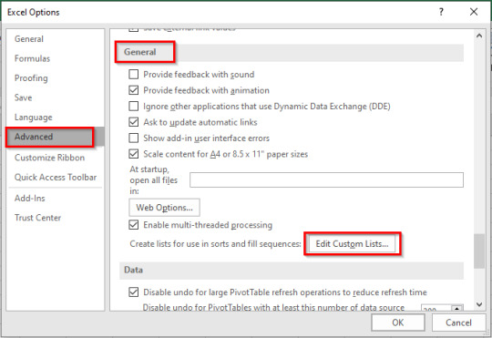
If you do not see the plus like symbol, that means you need to enable fill handle tool in Excel. To do so, go to File Tab > Options Button. In the ‘Excel Options’ dialog box that appears, check the option as highlighted in the image below.

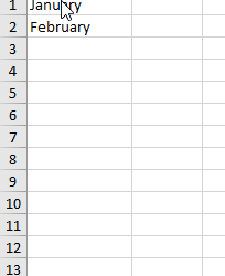
Once, the ‘Fill handle’ tool is activated, left-click on your mouse and drag it downwards till 12th row and then, release the mouse button. As a result, the excel would automatically list the months in the year. Refer to the demonstration below.

Excel somewhere knows that after February, comes March and so on. This is what is the Custom List Feature of Excel. Similarly, if you type the first two days of the week (Monday and Tuesday) and use the fill handle tool, you can quickly write all the seven days of the week.

Where is Custom List Feature in Excel

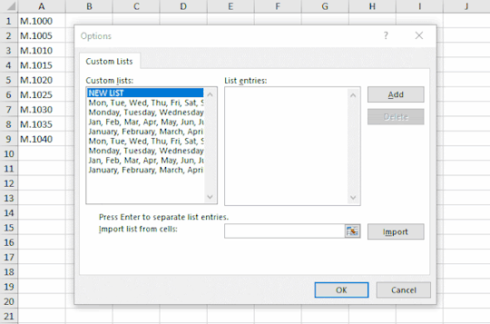
To navigate to the custom list feature in Excel, follow the undermentioned path. Go to File Tab > Options button > Advanced Option > General section > Edit Custom Lists ... Button.

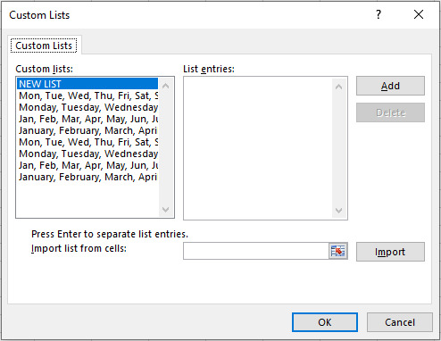
As soon as you click on this button, the ‘Custom List’ dialog box would appear on your screen where you can see the existing available custom lists and also create a new.

Let us now learn to create our own custom list.

Create our Own Custom Lists

Suppose you are working as a data entry operator in a company having thousands to products, each having a unique product code. You have to frequently insert this list of product codes in Excel. One way is to create this list somewhere (maybe in a notepad or word file) and then copy it from there and paste it in the cell each time you require it. Alternatively, you can create a custom list for it and then use it each time you need to insert a list of material codes by any of the following methods: Entering manually in ‘Custom List’ dialog boxUsing the ‘Import’ feature Manually Create a Custom List To manually create a custom list, navigate to the ‘Custom List’ dialog box using the path - File Tab > Options button > Advanced Option > General section > Edit Custom Lists ... Button. 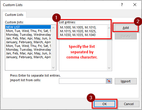Click anywhere inside the ‘List Entries’ section, and enter the list separated by comma characters and then click on the ‘Add’ button as shown in the image below:

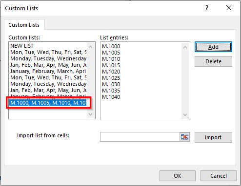
As soon as you click on the ‘Add’ button, the list would get added to the ‘Custom List’ section as highlighted in the image below:

Create List Using ‘Import’ Feature If you have a list of thousand values, creating the list manually is not a suggested technique. In that case, you can use the ‘Import’ button. A pre-requisite is that you need to have the list for once in Excel. Steps- Click on the ‘Import List from Cells’ input box and select the range of values. Once selected, click on the ‘Import’ button. As a result, the list would get added to the ‘Custom List’ section. Click on ‘OK’ button to exit.

Insert Custom List in Cell

Now, when creating a custom list in Excel is done, you can insert the custom list in cells in Excel. To do so, follow the below steps: Enter the first value of the list in the cell (in our case it is M.1000). Then, take your mouse cursor to the bottom-right corner of the cell, and the mouse cursor would change to a plus like a symbol (known as 'Fill Handle'). Once visible, left-click on your mouse and drag the mouse downwards to get the list as demonstrated below:

Create Custom Sorting Criteria in Excel

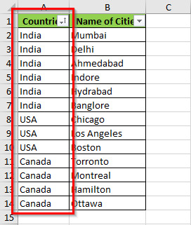
By default, you can sort the values/numbers/date in either ascending order or in the descending order. However, using the custom list in Excel, you can create your own customized sort in order to sort your list in order of this list. Let us take one example to understand this better. See the below image:

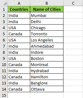
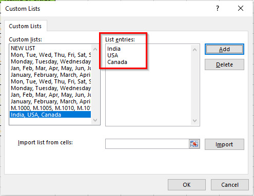
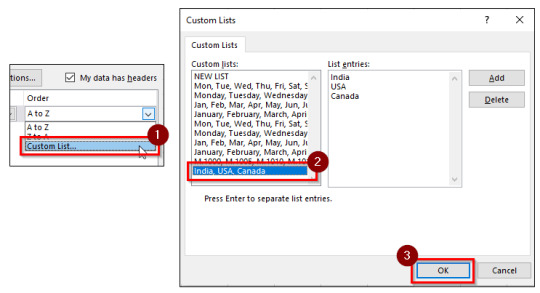
Suppose you want to sort the above list based on the countries in order - India, then the USA, and Canada. You can see that sorting using the in-built sort feature will not allow you to sort in this order. Instead, it would sort in either ascending order (Canada, India, USA) or in descending order (USA, India, Canada). However, to sort in an order other than ascending or descending order, firstly, we need to create a list in custom sorting order - India, USA, Canada. Refer to the image below:

Now, sort the dataset, using the steps below. Select the dataset A1:B14 and click on the ‘Sort’ button (under ‘Data’ tab > ‘Sort & Filter’ group). As a result, the ‘Sort’ dialog box would pop out on your screen.

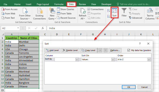
Before sorting your data, make sure that the ‘My data has headers’ checkbox is ticked. Under the ‘Sort by’ option, select the sorting column header as “Countries” and keep ‘Sort On’ as “Values”.

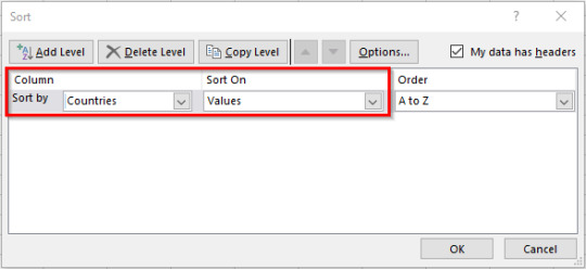
Under the ‘Order’ drop-down option, select ‘Custom Sort’ and as a result, the ‘Custom Lists’ dialog box would appear on your screen. Select the newly created Custom List (India, USA, Canada) and click on ‘OK’ to exit.

As a result, the custom list would appear in the ‘Order’ section of the ‘Sort’ dialog box. Finally, exit the ‘Sort’ dialog box by clicking on the ‘OK’ button. The excel would sort the dataset based on the newly created custom list as shown in the image below:

This brings us to the end of this blog. Share your views and comments in the comment section below. Read the full article

0 notes

excelunlocked-blog · 4 years

Text

How to Remove Leading Spaces in Excel

Has it happened with you that you export some data from some system and there are unwanted spaces before a number, text in Excel? Removing these spaces one by one manually is very time-consuming and irritating task that no one would like to do ideally. Then how to remove these unwanted leading spaces before a word in Excel? In this blog, we would unlock the technique to remove the leading spaces before a word in the excel worksheet. This can be done using both the Formula and Non-Formula-based approaches. This blog aims at unlocking both the ways. Let us take a small example to perform the same. 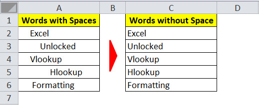Suppose we have a list of words. The words have blank space before them as shown in the screenshot below.

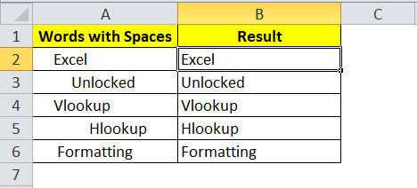
The requirement here is to remove the space before these texts and get the result as shown below :

There are three ways using which we can remove the extra space before any word in excel : =TRIM() Formula=SUBSTITUTE() FormulaUsing the "Find and Replace" Option (without formula) Let us understand each of the methods in detail.

Remove Leading Spaces Using formula =TRIM()

The Formula =TRIM() is used to remove multiple spaces between words in a sentence. Use the below formula (refer to the screenshot below). =TRIM(A2)

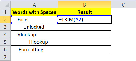
You can now see that the formula removed the extra spaces at the beginning of the word. Copy this formula to other cells in column B.

Remove Leading Spaces Using =SUBSTITUTE() Formula

This is also a formula-based approach. We would be using =SUBSTITUTE() formula to replace the spaces before a word/text in an excel. However, it is pertinent to note that, unlike =TRIM(), this formula will not be useful for removing additional spaces between two words in a sentence. Enter the following formula in cell B2 : =SUBSTITUTE(A2," ","")

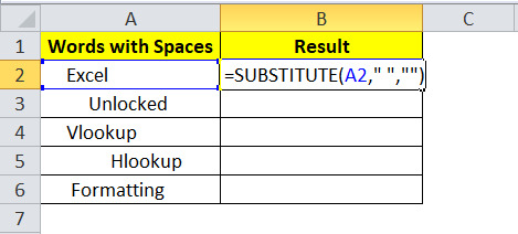
Explanation on the above formula: The formula would first take the value of cell A2 (denoted by the first attribute). After that, it would find spaces in that value (denoted by the second attribute- " "). And finally, the excel would replace the " " (i.e. space) with "" (i.e. blank) which is denoted by the third attribute of the formula. Copy this formula to other cells in column B.

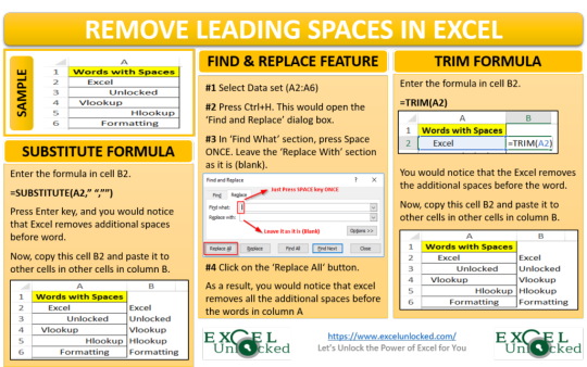
Using "Find and Replace" Option (without Formula)

This is the most simple method to remove additional spaces before any word in an excel. Unlike the above two methods, this is not a formula-based approach. Follow the below steps to remove the spaces in the beginning of the text: Select the cells which contain the text (from which spaces are to be removed)

Open the "Find and Replace" dialog box by pressing Ctrl+H on your keyboard.

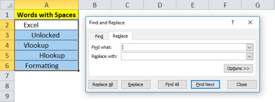
In the "Find What" section of this dialog box, just press the space button on your keyboard. This denotes that Excel should search/find for spaces in the selected cells.

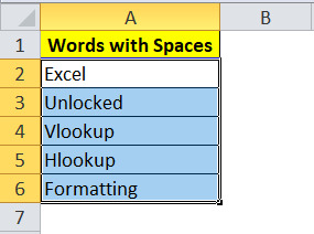
And do not enter anything in the "Replace with" section of this dialog box. Keep it as it is. This denotes that the value to be replaced with is blank/none. Now press the "Replace All" button. As a result, you can see that all the spaces at the beginning of the text get removed and you have a result as below :

This brings us to the end of this blog. Read the full article

0 notes

excelunlocked-blog · 4 years

Text

Insert Symbols and Special Characters in Excel

Most of the time, while working with Excel, you would be using either numbers or text in a cell. But do you know you can also insert symbols like (tick mark, cross mark, arrows, and thousands of such symbols) in excel? Excel also allows you to insert special characters like a trademark, copyright, registered symbols, and many more. In this blog, we would unlock a few ways that you can use to insert the symbols and special characters in an Excel cell.

Ways To Insert Symbols in Excel

The easiest way to insert a symbol or a special character in Excel is to search for that symbol in the search engine, copy it (Ctrl+C), and finally paste it (Ctrl+V) in the cell to which you want it. To paste the symbol such that it matches the formatting of your cell, use Ctrl + Shift + V instead of simple Ctrl + V. However, unlike the above method, excel has an in-built symbol option from where you can insert the symbols in Excel. In the upcoming section, we would learn to insert the symbols or the special characters using these in-built options.

Where is This Built-In Option?

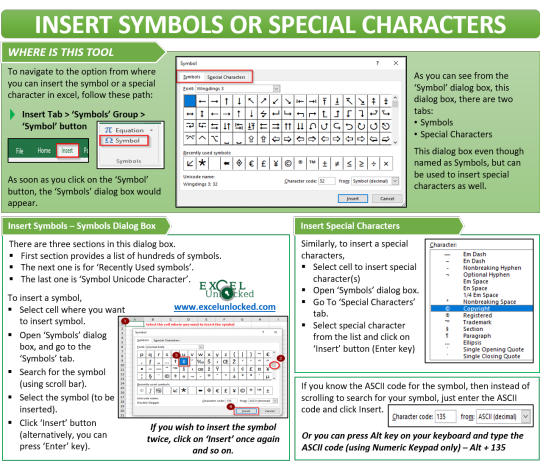
To navigate to the in-built excel symbols option, follow the below path. ‘Insert’ Tab > ‘Symbols’ group > ‘Symbol’ button

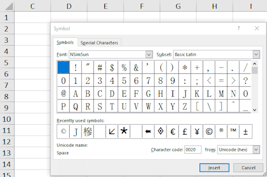
Insert Symbols Using ‘Symbols’ Options

Even though the name of the option is given as ‘Symbols’, however, you can use the same option to insert any special character in Excel. Now, select the cell, and then navigate to the ‘Symbol’ option, as shown in the above section, and click on the ‘Symbol’ button.

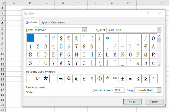
As a result, the ‘Symbol’ dialog box would appear. As you can see, there are two tabs, one for ‘Symbols’ and another for ‘Special Characters’.

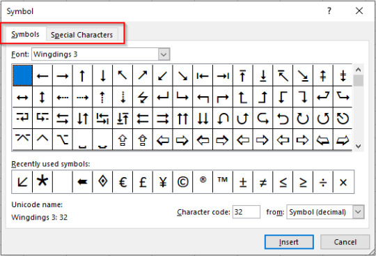
There are basically, three sections in this dialog box. The first section provides a list of hundreds of symbols. The next section is for ‘Recently used symbols’ and the last one is ‘Symbol Unicode Character’. To insert any symbol, search for the symbol from the list. Then select it and then click on the ‘Insert’ button once. Alternatively, you can press the ‘Enter’ key on your keyboard instead of using the ‘Insert’ button.

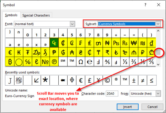
If you click ‘Insert’ twice, then excel would insert two symbols in the same cell. As you can see, the list of symbols is quite large, and searching for your symbol using the scroll bar is not an easy task. To mitigate this, you can use the options in the ‘Subset’ drop-down button which logically groups the symbols. For example, ‘Currency Symbol’ subset groups all the currencies and so on.

Even you can change the font to Wingdings, Webdings, to get a whole range of exciting symbols. You can insert tick marks, cross marks using the Wingdings font.

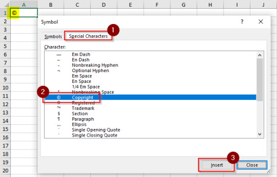
Insert Special Characters in Excel

Excel has pre-provided some of the special characters like a trademark, registered, copyright, etc. You can find these in the tab named ‘Special Characters’ (shown below). Select the character that you want to insert and click the ‘Insert’ button as shown in the image below:

Insert Symbol Using Code

As we saw in the previous sections, to insert a symbol, you need to scroll down a lot and search for the required symbol. However, searching for a symbol that you want to use frequently and inserting it using the above method is not worthy to do. In order to get rid of this tiresome task, you can use the character code of the symbol. It is visible on the bottom right section of this dialog box.

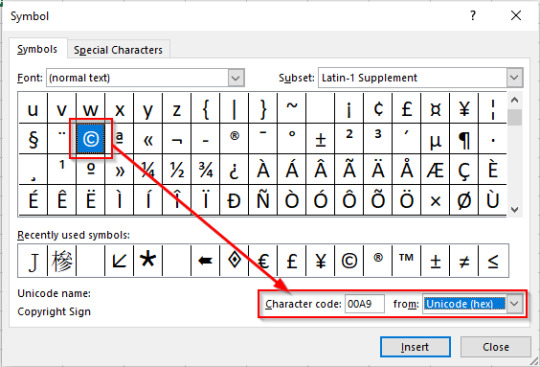
Search for the symbol to insert from the list, click it, and check its code. Note this code somewhere and in the future, just enter this code there and click Insert to insert it quickly. You can get the character code in three encodings - Unicode (hex), ASCII (hex) and ASCII (decimal). For example, the copyright symbol code under the three encodings are like: Unicode (hex) - 00A9ASCII (decimal) - 169ASCII (hex) - 00A9 A pictorial demonstration to insert the symbol using the character code:

If you know the ASCII character code for a symbol, you can quickly insert a symbol using the Alt key followed by the character code on the numeric keypad ONLY. For Example, Alt + 169 will quickly insert a copyright symbol (without navigating to the symbols dialog box. This brings to the end of this blog. Share your views and comments in the comment section below. Read the full article

0 notes