monuonrise

[monuonrise]

Running a k-means Cluster Analysis:

Machine Learning for Data Analysis

Week 4: Running a k-means Cluster Analysis

A k-means cluster analysis was conducted to identify underlying subgroups of countries based on their similarity of responses on 7 variables that represent characteristics that could have an impact on internet use rates. Clustering variables included quantitative variables measuring income per person, employment rate, female employment rate, polity score, alcohol consumption, life expectancy, and urban rate. All clustering variables were standardized to have a mean of 0 and a standard deviation of 1.

Because the GapMinder dataset which I am using is relatively small (N < 250), I have not split the data into test and training sets. A series of k-means cluster analyses were conducted on the training data specifying k=1-9 clusters, using Euclidean distance. The variance in the clustering variables that was accounted for by the clusters (r-square) was plotted for each of the nine cluster solutions in an elbow curve to provide guidance for choosing the number of clusters to interpret.

Load the data, set the variables to numeric, and clean the data of NA values

In [1]:''' Code for Peer-graded Assignments: Running a k-means Cluster Analysis Course: Data Management and Visualization Specialization: Data Analysis and Interpretation ''' import pandas as pd import numpy as np import matplotlib.pyplot as plt import statsmodels.formula.api as smf import statsmodels.stats.multicomp as multi from sklearn.cross_validation import train_test_split from sklearn import preprocessing from sklearn.cluster import KMeans data = pd.read_csv('c:/users/greg/desktop/gapminder.csv', low_memory=False) data['internetuserate'] = pd.to_numeric(data['internetuserate'], errors='coerce') data['incomeperperson'] = pd.to_numeric(data['incomeperperson'], errors='coerce') data['employrate'] = pd.to_numeric(data['employrate'], errors='coerce') data['femaleemployrate'] = pd.to_numeric(data['femaleemployrate'], errors='coerce') data['polityscore'] = pd.to_numeric(data['polityscore'], errors='coerce') data['alcconsumption'] = pd.to_numeric(data['alcconsumption'], errors='coerce') data['lifeexpectancy'] = pd.to_numeric(data['lifeexpectancy'], errors='coerce') data['urbanrate'] = pd.to_numeric(data['urbanrate'], errors='coerce') sub1 = data.copy() data_clean = sub1.dropna()

Subset the clustering variables

In [2]:cluster = data_clean[['incomeperperson','employrate','femaleemployrate','polityscore', 'alcconsumption', 'lifeexpectancy', 'urbanrate']] cluster.describe()

Out[2]:incomeperpersonemployratefemaleemployratepolityscorealcconsumptionlifeexpectancyurbanratecount150.000000150.000000150.000000150.000000150.000000150.000000150.000000mean6790.69585859.26133348.1006673.8933336.82173368.98198755.073200std9861.86832710.38046514.7809996.2489165.1219119.90879622.558074min103.77585734.90000212.400000-10.0000000.05000048.13200010.40000025%592.26959252.19999939.599998-1.7500002.56250062.46750036.41500050%2231.33485558.90000248.5499997.0000006.00000072.55850057.23000075%7222.63772165.00000055.7250009.00000010.05750076.06975071.565000max39972.35276883.19999783.30000310.00000023.01000083.394000100.000000

Standardize the clustering variables to have mean = 0 and standard deviation = 1

In [3]:clustervar=cluster.copy() clustervar['incomeperperson']=preprocessing.scale(clustervar['incomeperperson'].astype('float64')) clustervar['employrate']=preprocessing.scale(clustervar['employrate'].astype('float64')) clustervar['femaleemployrate']=preprocessing.scale(clustervar['femaleemployrate'].astype('float64')) clustervar['polityscore']=preprocessing.scale(clustervar['polityscore'].astype('float64')) clustervar['alcconsumption']=preprocessing.scale(clustervar['alcconsumption'].astype('float64')) clustervar['lifeexpectancy']=preprocessing.scale(clustervar['lifeexpectancy'].astype('float64')) clustervar['urbanrate']=preprocessing.scale(clustervar['urbanrate'].astype('float64'))

Split the data into train and test sets

In [4]:clus_train, clus_test = train_test_split(clustervar, test_size=.3, random_state=123)

Perform k-means cluster analysis for 1-9 clusters

In [5]:from scipy.spatial.distance import cdist clusters = range(1,10) meandist = [] for k in clusters: model = KMeans(n_clusters = k) model.fit(clus_train) clusassign = model.predict(clus_train) meandist.append(sum(np.min(cdist(clus_train, model.cluster_centers_, 'euclidean'), axis=1)) / clus_train.shape[0])

Plot average distance from observations from the cluster centroid to use the Elbow Method to identify number of clusters to choose

In [6]:plt.plot(clusters, meandist) plt.xlabel('Number of clusters') plt.ylabel('Average distance') plt.title('Selecting k with the Elbow Method') plt.show()

64.media.tumblr.com

Interpret 3 cluster solution

In [7]:model3 = KMeans(n_clusters=4) model3.fit(clus_train) clusassign = model3.predict(clus_train)

Plot the clusters

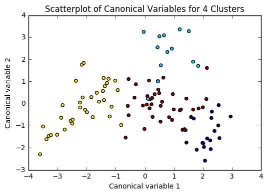
In [8]:from sklearn.decomposition import PCA pca_2 = PCA(2) plt.figure() plot_columns = pca_2.fit_transform(clus_train) plt.scatter(x=plot_columns[:,0], y=plot_columns[:,1], c=model3.labels_,) plt.xlabel('Canonical variable 1') plt.ylabel('Canonical variable 2') plt.title('Scatterplot of Canonical Variables for 4 Clusters') plt.show()

64.media.tumblr.com

Begin multiple steps to merge cluster assignment with clustering variables to examine cluster variable means by cluster.

Create a unique identifier variable from the index for the cluster training data to merge with the cluster assignment variable.

In [9]:clus_train.reset_index(level=0, inplace=True)

Create a list that has the new index variable

In [10]:cluslist = list(clus_train['index'])

Create a list of cluster assignments

In [11]:labels = list(model3.labels_)

Combine index variable list with cluster assignment list into a dictionary

In [12]:newlist = dict(zip(cluslist, labels)) print (newlist) {2: 1, 4: 2, 6: 0, 10: 0, 11: 3, 14: 2, 16: 3, 17: 0, 19: 2, 22: 2, 24: 3, 27: 3, 28: 2, 29: 2, 31: 2, 32: 0, 35: 2, 37: 3, 38: 2, 39: 3, 42: 2, 45: 2, 47: 1, 53: 3, 54: 3, 55: 1, 56: 3, 58: 2, 59: 3, 63: 0, 64: 0, 66: 3, 67: 2, 68: 3, 69: 0, 70: 2, 72: 3, 77: 3, 78: 2, 79: 2, 80: 3, 84: 3, 88: 1, 89: 1, 90: 0, 91: 0, 92: 0, 93: 3, 94: 0, 95: 1, 97: 2, 100: 0, 102: 2, 103: 2, 104: 3, 105: 1, 106: 2, 107: 2, 108: 1, 113: 3, 114: 2, 115: 2, 116: 3, 123: 3, 126: 3, 128: 3, 131: 2, 133: 3, 135: 2, 136: 0, 139: 0, 140: 3, 141: 2, 142: 3, 144: 0, 145: 1, 148: 3, 149: 2, 150: 3, 151: 3, 152: 3, 153: 3, 154: 3, 158: 3, 159: 3, 160: 2, 173: 0, 175: 3, 178: 3, 179: 0, 180: 3, 183: 2, 184: 0, 186: 1, 188: 2, 194: 3, 196: 1, 197: 2, 200: 3, 201: 1, 205: 2, 208: 2, 210: 1, 211: 2, 212: 2}

Convert newlist dictionary to a dataframe

In [13]:newclus = pd.DataFrame.from_dict(newlist, orient='index') newclus

Out[13]:0214260100113142163170192222243273282292312320352373382393422452471533543551563582593630......145114831492150315131523153315431583159316021730175317831790180318321840186118821943196119722003201120522082210121122122

105 rows × 1 columns

Rename the cluster assignment column

In [14]:newclus.columns = ['cluster']

Repeat previous steps for the cluster assignment variable

Create a unique identifier variable from the index for the cluster assignment dataframe to merge with cluster training data

In [15]:newclus.reset_index(level=0, inplace=True)

Merge the cluster assignment dataframe with the cluster training variable dataframe by the index variable

In [16]:merged_train = pd.merge(clus_train, newclus, on='index') merged_train.head(n=100)

Out[16]:indexincomeperpersonemployratefemaleemployratepolityscorealcconsumptionlifeexpectancyurbanratecluster0159-0.393486-0.0445910.3868770.0171271.843020-0.0160990.79024131196-0.146720-1.591112-1.7785290.498818-0.7447360.5059900.6052111270-0.6543650.5643511.0860520.659382-0.727105-0.481382-0.2247592329-0.6791572.3138522.3893690.3382550.554040-1.880471-1.9869992453-0.278924-0.634202-0.5159410.659382-0.1061220.4469570.62033335153-0.021869-1.020832-0.4073320.9805101.4904110.7233920.2778493635-0.6665191.1636281.004595-0.785693-0.715352-2.084304-0.7335932714-0.6341100.8543230.3733010.177691-1.303033-0.003846-1.24242828116-0.1633940.119726-0.3394510.338255-1.1659070.5304950.67993439126-0.630263-1.446126-0.3055100.6593823.1711790.033923-0.592152310123-0.163655-0.460219-0.8010420.980510-0.6448300.444628-0.560127311106-0.640452-0.2862350.1153530.659382-0.247166-2.104758-1.317152212142-0.635480-0.808186-0.7874660.0171271.155433-1.731823-0.29859331389-0.615980-2.113062-2.423400-0.625129-1.2442650.0060770.512695114160-0.6564731.9852172.199302-1.1068200.620643-1.371039-1.63383921556-0.430694-0.102586-0.2240530.659382-0.5547190.3254460.250272316180-0.559059-0.402224-0.6041870.338255-1.1776610.603401-1.777949317133-0.419521-1.668438-0.7331610.3382551.032020-0.659900-0.81098631831-0.618282-0.0155940.061048-1.2673840.211226-1.7590620.075026219171.801349-1.030498-0.4344840.6593820.7029191.1165791.8808550201450.447771-0.827517-1.731013-1.909640-1.1561120.4042250.7359771211000.974856-0.034925-0.0068330.6593822.4150301.1806761.173646022178-0.309804-1.755430-0.9368040.8199460.653945-1.6388680.2520513231732.6193200.3033760.217174-0.946256-1.0346581.2296851.99827802459-0.056177-0.2669040.2714790.8199462.0408730.5916550.63990432568-0.562821-0.3538960.0271070.338255-0.0316830.481486-0.1037773261080.111383-1.030498-1.690284-1.749076-1.3167450.5879080.999290127212-0.6582520.7286690.678765-0.464565-0.364702-1.781946-0.78874722819-0.6525281.1926250.6855540.498818-0.928876-1.306335-0.617060229188-0.662484-0.4505530.135717-1.106820-0.672255-0.147127-1.2726732..............................70140-0.594402-0.044591-0.8214060.819946-0.3157280.5125720.074137371148-0.0905570.052066-0.3190860.8199460.0936890.7235950.80625437211-0.4523170.1583900.549792-1.7490761.2768870.177913-0.140250373641.636776-0.779188-0.1697480.8199461.1084191.2715050.99128407484-0.117682-1.156153-0.5295180.9805101.8214720.5500380.5527263751750.604211-0.3248980.0882000.9805101.5903171.048938-0.287918376197-0.481087-0.0735890.393665-2.070203-0.356866-0.404628-0.287029277183-0.506714-0.808186-0.067926-2.070203-0.347071-2.051902-1.340281278210-0.628790-1.958410-1.887139-0.946256-1.297156-0.353290-1.08675317954-0.5150780.042400-0.1765360.1776910.5109430.6733710.467327380114-0.6661982.2945212.111056-0.625129-1.077755-0.229248-1.1365692814-0.5503841.5889211.445822-0.946256-0.245207-1.8114130.072358282911.575455-0.769523-0.1154430.980510-0.8426821.2795041.62732708377-0.5015740.332373-0.2783580.6593820.0545110.221758-0.28880838466-0.265535-0.0252600.305419-0.1434370.516820-0.6358011.332879385921.240375-1.243145-0.8349830.9805100.5677521.3035020.5785230862011.4545511.540592-0.733161-1.909640-1.2344700.7659211.014413187105-0.004485-1.281808-1.7513770.498818-0.8857790.3704051.418278188205-0.593947-0.1702460.305419-2.070203-0.629158-0.070373-0.8118762891540.504036-0.1605810.1696570.9805101.3846291.0649370.19511839045-0.6307520.061732-0.678856-0.625129-0.068902-1.377621-0.27991229197-0.6432031.3472771.2557550.498818-0.576267-1.199710-1.488839292632.067368-0.1992430.3597250.9805101.2298731.1133390.365916093211-0.6469130.1680550.3665130.498818-0.638953-2.020815-0.874146294158-0.422620-0.943506-0.2919340.8199461.8273490.505990-0.037060395135-0.6635950.2453810.4411820.338255-0.862272-0.018934-1.68276529679-0.6744750.6416770.1221410.338255-0.572349-2.111239-1.1223362971790.882197-0.653534-0.4344840.9805100.9810881.2578350.980609098149-0.6151691.0766361.4118810.017127-0.623282-0.626890-1.891814299113-0.464904-2.354706-1.4459120.8199460.4149550.5938830.5260393

100 rows × 9 columns

Cluster frequencies

In [17]:merged_train.cluster.value_counts()

Out[17]:3 39 2 35 0 18 1 13 Name: cluster, dtype: int64

Calculate clustering variable means by cluster

In [18]:clustergrp = merged_train.groupby('cluster').mean() print ("Clustering variable means by cluster") clustergrp Clustering variable means by cluster

Out[18]:indexincomeperpersonemployratefemaleemployratepolityscorealcconsumptionlifeexpectancyurbanratecluster093.5000001.846611-0.1960210.1010220.8110260.6785411.1956961.0784621117.461538-0.154556-1.117490-1.645378-1.069767-1.0827280.4395570.5086582100.657143-0.6282270.8551520.873487-0.583841-0.506473-1.034933-0.8963853107.512821-0.284648-0.424778-0.2000330.5317550.6146160.2302010.164805

Validate clusters in training data by examining cluster differences in internetuserate using ANOVA. First, merge internetuserate with clustering variables and cluster assignment data

In [19]:internetuserate_data = data_clean['internetuserate']

Split internetuserate data into train and test sets

In [20]:internetuserate_train, internetuserate_test = train_test_split(internetuserate_data, test_size=.3, random_state=123) internetuserate_train1=pd.DataFrame(internetuserate_train) internetuserate_train1.reset_index(level=0, inplace=True) merged_train_all=pd.merge(internetuserate_train1, merged_train, on='index') sub5 = merged_train_all[['internetuserate', 'cluster']].dropna()

In [21]:internetuserate_mod = smf.ols(formula='internetuserate ~ C(cluster)', data=sub5).fit() internetuserate_mod.summary()

Out[21]:

OLS Regression ResultsDep. Variable:internetuserateR-squared:0.679Model:OLSAdj. R-squared:0.669Method:Least SquaresF-statistic:71.17Date:Thu, 12 Jan 2017Prob (F-statistic):8.18e-25Time:20:59:17Log-Likelihood:-436.84No. Observations:105AIC:881.7Df Residuals:101BIC:892.3Df Model:3Covariance Type:nonrobustcoefstd errtP>|t|[95.0% Conf. Int.]Intercept75.20683.72720.1770.00067.813 82.601C(cluster)[T.1]-46.95175.756-8.1570.000-58.370 -35.534C(cluster)[T.2]-66.56684.587-14.5130.000-75.666 -57.468C(cluster)[T.3]-39.48604.506-8.7630.000-48.425 -30.547Omnibus:5.290Durbin-Watson:1.727Prob(Omnibus):0.071Jarque-Bera (JB):4.908Skew:0.387Prob(JB):0.0859Kurtosis:3.722Cond. No.5.90

Means for internetuserate by cluster

In [22]:m1= sub5.groupby('cluster').mean() m1

Out[22]:internetuseratecluster075.206753128.25501828.639961335.720760

Standard deviations for internetuserate by cluster

In [23]:m2= sub5.groupby('cluster').std() m2

Out[23]:internetuseratecluster014.093018121.75775228.399554319.057835

In [24]:mc1 = multi.MultiComparison(sub5['internetuserate'], sub5['cluster']) res1 = mc1.tukeyhsd() res1.summary()

Out[24]:

Multiple Comparison of Means - Tukey HSD,FWER=0.05group1group2meandifflowerupperreject01-46.9517-61.9887-31.9148True02-66.5668-78.5495-54.5841True03-39.486-51.2581-27.7139True12-19.6151-33.0335-6.1966True137.4657-5.76520.6965False2327.080817.461736.6999True

The elbow curve was inconclusive, suggesting that the 2, 4, 6, and 8-cluster solutions might be interpreted. The results above are for an interpretation of the 4-cluster solution.

In order to externally validate the clusters, an Analysis of Variance (ANOVA) was conducting to test for significant differences between the clusters on internet use rate. A tukey test was used for post hoc comparisons between the clusters. Results indicated significant differences between the clusters on internet use rate (F=71.17, p<.0001). The tukey post hoc comparisons showed significant differences between clusters on internet use rate, with the exception that clusters 0 and 2 were not significantly different from each other. Countries in cluster 1 had the highest internet use rate (mean=75.2, sd=14.1), and cluster 3 had the lowest internet use rate (mean=8.64, sd=8.40).

[monuonrise]

Running a Lasso Regression Analysis

import pandas as pd import numpy as np import matplotlib.pylab as plt from sklearn.cross_validation import train_test_split from sklearn.linear_model import LassoLarsCV

Load the dataset

data = pd.read_csv("gapminder_ghana_updated.csv")

#

DATA MANAGEMENT

CONVERTING SOME QUANTITATIVE VARIABLES INTO CATEGORICAL VARIABLES TO GET FEEL

OF LASSO REGRESSION

#

data_clean = data.dropna()

check minimum and maximum values of totalpopulationfemale and create categorical

variable out of it

print(data_clean["totalpopulationfemale"].describe())

def totalpopulationfemaleGrp(row): if row["totalpopulationfemale"]<=7758806: return 0 elif row["totalpopulationfemale"] > 7758806: return 1

data_clean["totalpopulationfemaleGrp"] = data_clean.apply(lambda row:totalpopulationfemaleGrp(row), axis =1 )

check values in totalpopulationfemaleGrp

checktotFemPop = data_clean["totalpopulationfemaleGrp"].value_counts(sort=False, dropna=True) print(checktotFemPop)

check minimum and maximum values of malebloodpressure and create categorical

variable out of it

print(data_clean["malebloodpressure"].describe())

def malebloodpressureGrp(row): if row["malebloodpressure"]<=129: return 0 elif row["malebloodpressure"] > 129: return 1

data_clean["malebloodpressureGrp"] = data_clean.apply(lambda row:totalpopulationfemaleGrp(row), axis =1 )

check values ink totalpopulationfemaleGrp

checkmaleblood = data_clean["malebloodpressureGrp"].value_counts(sort=False, dropna=True) print(checkmaleblood)

creating categorical explanatory variables out of exports

def exportsCatGrp (row): if row["exports"] <=40: return 0 elif row["exports"] >40: return 1

data_clean["exportsCatGrp"] = data_clean.apply(lambda row:exportsCatGrp(row), axis =1)

creating a categorical explanatry variable out of incomeperperson

def incomeLevelGrp (row): if row["incomeperperson"] <=2200: return 0 elif row["incomeperperson"] >2200: return 1

data_clean["incomeLevelGrp"] = data_clean.apply(lambda row:incomeLevelGrp(row), axis =1)

#

END OF DATA MANAGEMENT

#

predvar= data_clean[['incomeLevelGrp','exportsCatGrp','malebloodpressureGrp', 'totalpopulationfemaleGrp','inflation','agriculture','democracyscore', 'agriculturalland','aidreceived','aidreceivedperperson','realgdppercapita', 'femalebloodpressure','malebodymassindex','femalebodymassindex','underfivemortality', 'totalfertilityrate','cholesterolinmen','cholesterolinwomen','crudebirthrate', 'deadkidsperwoman','externaldebtstocks','energyuse']]

target = data_clean.lifeexpectancy

standardize predictors to have mean=0 and sd=1

predictors=predvar.copy() from sklearn import preprocessing predictors['incomeLevelGrp']=preprocessing.scale(predictors['incomeLevelGrp'].astype('float64')) predictors['exportsCatGrp']=preprocessing.scale(predictors['exportsCatGrp'].astype('float64')) predictors['inflation']=preprocessing.scale(predictors['inflation'].astype('float64')) predictors['agriculture']=preprocessing.scale(predictors['agriculture'].astype('float64')) predictors['democracyscore']=preprocessing.scale(predictors['democracyscore'].astype('float64')) predictors['agriculturalland']=preprocessing.scale(predictors['agriculturalland'].astype('float64')) predictors['aidreceived']=preprocessing.scale(predictors['aidreceived'].astype('float64')) predictors['aidreceivedperperson']=preprocessing.scale(predictors['aidreceivedperperson'].astype('float64')) predictors['realgdppercapita']=preprocessing.scale(predictors['realgdppercapita'].astype('float64')) predictors['malebloodpressureGrp']=preprocessing.scale(predictors['malebloodpressureGrp'].astype('float64')) predictors['femalebloodpressure']=preprocessing.scale(predictors['femalebloodpressure'].astype('float64')) predictors['malebodymassindex']=preprocessing.scale(predictors['malebodymassindex'].astype('float64')) predictors['femalebodymassindex']=preprocessing.scale(predictors['femalebodymassindex'].astype('float64')) predictors['underfivemortality']=preprocessing.scale(predictors['underfivemortality'].astype('float64')) predictors['totalfertilityrate']=preprocessing.scale(predictors['totalfertilityrate'].astype('float64')) predictors['cholesterolinmen']=preprocessing.scale(predictors['cholesterolinmen'].astype('float64')) predictors['cholesterolinwomen']=preprocessing.scale(predictors['cholesterolinwomen'].astype('float64')) predictors['crudebirthrate']=preprocessing.scale(predictors['crudebirthrate'].astype('float64')) predictors['deadkidsperwoman']=preprocessing.scale(predictors['deadkidsperwoman'].astype('float64')) predictors['externaldebtstocks']=preprocessing.scale(predictors['externaldebtstocks'].astype('float64')) predictors['energyuse']=preprocessing.scale(predictors['energyuse'].astype('float64')) predictors['totalpopulationfemaleGrp']=preprocessing.scale(predictors['totalpopulationfemaleGrp'].astype('float64'))

split data into train and test sets

pred_train, pred_test, tar_train, tar_test = train_test_split(predictors, target, test_size=.3, random_state=123)

specify the lasso regression model

model=LassoLarsCV(cv=10, precompute=False).fit(pred_train,tar_train)

print variable names and regression coefficients

dict(zip(predictors.columns, model.coef_))

plot coefficient progression

m_log_alphas = -np.log10(model.alphas_) ax = plt.gca() plt.plot(m_log_alphas, model.coef_path_.T) plt.axvline(-np.log10(model.alpha_), linestyle='--', color='k', label='alpha CV') plt.ylabel('Regression Coefficients') plt.xlabel('-log(alpha)') plt.title('Regression Coefficients Progression for Lasso Paths')

plot mean square error for each fold

m_log_alphascv = -np.log10(model.cv_alphas_) plt.figure() plt.plot(m_log_alphascv, model.cv_mse_path_, ':') plt.plot(m_log_alphascv, model.cv_mse_path_.mean(axis=-1), 'k', label='Average across the folds', linewidth=2) plt.axvline(-np.log10(model.alpha_), linestyle='--', color='k', label='alpha CV') plt.legend() plt.xlabel('-log(alpha)') plt.ylabel('Mean squared error') plt.title('Mean squared error on each fold')

MSE from training and test data

from sklearn.metrics import mean_squared_error train_error = mean_squared_error(tar_train, model.predict(pred_train)) test_error = mean_squared_error(tar_test, model.predict(pred_test)) print ('training data MSE') print(train_error) print ('test data MSE') print(test_error)

R-square from training and test data

rsquared_train=model.score(pred_train,tar_train) rsquared_test=model.score(pred_test,tar_test) print ('training data R-square') print(rsquared_train) print ('test data R-square') print(rsquared_test)

[monuonrise]

Running a Random Forest

import pandas as pd

import numpy as np

import matplotlib.pylab as plt

from sklearn.model_selection import train_test_split, cross_val_score

from sklearn.ensemble import RandomForestClassifier,

ExtraTreesClassifier

from sklearn.manifold import MDS

from sklearn.metrics.pairwise import pairwise_distances

from sklearn.metrics import accuracy_score

import seaborn as sns

%matplotlib inline

rnd_state = 4536 data = pd.read_csv('Data\winequality-red.csv', sep=';') data.info()

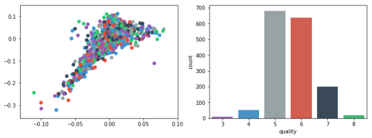
RangeIndex: 1599 entries, 0 to 1598 Data columns (total 12 columns): fixed acidity 1599 non-null float64 volatile acidity 1599 non-null float64 citric acid 1599 non-null float64 residual sugar 1599 non-null float64 chlorides 1599 non-null float64 free sulfur dioxide 1599 non-null float64 total sulfur dioxide 1599 non-null float64 density 1599 non-null float64 pH 1599 non-null float64 sulphates 1599 non-null float64 alcohol 1599 non-null float64 quality 1599 non-null int64 dtypes: float64(11), int64(1) memory usage: 150.0 KB data.head() fixed acidity volatile acidity citric acid residual sugar chlorides free sulfur dioxide total sulfur dioxide density pH sulphates alcohol quality 0 7.4 0.70 0.00 1.9 0.076 11.0 34.0 0.9978 3.51 0.56 9.4 5 1 7.8 0.88 0.00 2.6 0.098 25.0 67.0 0.9968 3.20 0.68 9.8 5 2 7.8 0.76 0.04 2.3 0.092 15.0 54.0 0.9970 3.26 0.65 9.8 5 3 11.2 0.28 0.56 1.9 0.075 17.0 60.0 0.9980 3.16 0.58 9.8 6 4 7.4 0.70 0.00 1.9 0.076 11.0 34.0 0.9978 3.51 0.56 9.4 5 data.describe() fixed acidity volatile acidity citric acid residual sugar chlorides free sulfur dioxide total sulfur dioxide density pH sulphates alcohol quality count 1599.000000 1599.000000 1599.000000 1599.000000 1599.000000 1599.000000 1599.000000 1599.000000 1599.000000 1599.000000 1599.000000 1599.000000 mean 8.319637 0.527821 0.270976 2.538806 0.087467 15.874922 46.467792 0.996747 3.311113 0.658149 10.422983 5.636023 std 1.741096 0.179060 0.194801 1.409928 0.047065 10.460157 32.895324 0.001887 0.154386 0.169507 1.065668 0.807569 min 4.600000 0.120000 0.000000 0.900000 0.012000 1.000000 6.000000 0.990070 2.740000 0.330000 8.400000 3.000000 25% 7.100000 0.390000 0.090000 1.900000 0.070000 7.000000 22.000000 0.995600 3.210000 0.550000 9.500000 5.000000 50% 7.900000 0.520000 0.260000 2.200000 0.079000 14.000000 38.000000 0.996750 3.310000 0.620000 10.200000 6.000000 75% 9.200000 0.640000 0.420000 2.600000 0.090000 21.000000 62.000000 0.997835 3.400000 0.730000 11.100000 6.000000 max 15.900000 1.580000 1.000000 15.500000 0.611000 72.000000 289.000000 1.003690 4.010000 2.000000 14.900000 8.000000 For visualization purposes, the number of dimensions was reduced to two by applying MDS method with cosine distance. The plot illustrates that our classes are not clearly divided into parts.

model = MDS(random_state=rnd_state, n_components=2, dissimilarity='precomputed') %time representation = model.fit_transform(pairwise_distances(data.iloc[:, :11], metric='cosine')) Wall time: 38.7 s colors = ["#9b59b6", "#3498db", "#95a5a6", "#e74c3c", "#34495e", "#2ecc71"] plt.figure(figsize=(12, 4))

plt.subplot(121) plt.scatter(representation[:, 0], representation[:, 1], c=colors)

plt.subplot(122) sns.countplot(x='quality', data=data, palette=sns.color_palette(colors));

predictors = data.iloc[:, :11] target = data.quality

In [8]:(predictors_train, predictors_test, target_train, target_test) = train_test_split(predictors, target, test_size = .3, random_state = rnd_state)

RandomForest classifier

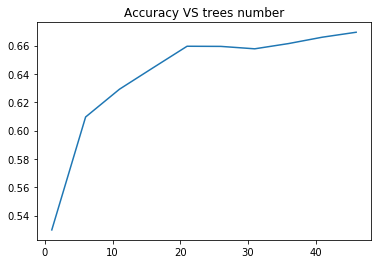
In [9]:list_estimators = list(range(1, 50, 5)) rf_scoring = [] for n_estimators in list_estimators: classifier = RandomForestClassifier(random_state = rnd_state, n_jobs =-1, class_weight='balanced', n_estimators=n_estimators) score = cross_val_score(classifier, predictors_train, target_train, cv=5, n_jobs=-1, scoring = 'accuracy') rf_scoring.append(score.mean())

In [10]:plt.plot(list_estimators, rf_scoring) plt.title('Accuracy VS trees number');

predictors = data.iloc[:, :11] target = data.quality

In [8]:(predictors_train, predictors_test, target_train, target_test) = train_test_split(predictors, target, test_size = .3, random_state = rnd_state)

RandomForest classifier

In [9]:list_estimators = list(range(1, 50, 5)) rf_scoring = [] for n_estimators in list_estimators: classifier = RandomForestClassifier(random_state = rnd_state, n_jobs =-1, class_weight='balanced', n_estimators=n_estimators) score = cross_val_score(classifier, predictors_train, target_train, cv=5, n_jobs=-1, scoring = 'accuracy') rf_scoring.append(score.mean())

In [10]:plt.plot(list_estimators, rf_scoring) plt.title('Accuracy VS trees number');

classifier = RandomForestClassifier(random_state = rnd_state, n_jobs =-1, class_weight='balanced', n_estimators=20) classifier.fit(predictors_train, target_train)

Out[11]:RandomForestClassifier(bootstrap=True, class_weight='balanced', criterion='gini', max_depth=None, max_features='auto', max_leaf_nodes=None, min_impurity_decrease=0.0, min_impurity_split=None, min_samples_leaf=1, min_samples_split=2, min_weight_fraction_leaf=0.0, n_estimators=20, n_jobs=-1, oob_score=False, random_state=4536, verbose=0, warm_start=False)

In [12]:prediction = classifier.predict(predictors_test)

In [13]:print('Confusion matrix:\n', pd.crosstab(target_test, prediction, colnames=['Predicted'], rownames=['Actual'], margins=True)) print('\nAccuracy: ', accuracy_score(target_test, prediction)) Confusion matrix: Predicted 3 4 5 6 7 All Actual 3 0 0 3 0 0 3 4 0 1 9 6 0 16 5 2 1 166 41 3 213 6 0 0 46 131 14 191 7 0 0 5 25 23 53 8 0 0 0 3 1 4 All 2 2 229 206 41 480 Accuracy: 0.66875

In [14]:feature_importance = pd.Series(classifier.feature_importances_, index=data.columns.values[:11]).sort_values(ascending=False) feature_importance

volatile acidity 0.133023 alcohol 0.130114 sulphates 0.129498 citric acid 0.106427 total sulfur dioxide 0.094647 chlorides 0.086298 density 0.079843 pH 0.066566 residual sugar 0.061344 fixed acidity 0.058251 free sulfur dioxide 0.053990 dtype: float64

In [15]:et_scoring = [] for n_estimators in list_estimators: classifier = ExtraTreesClassifier(random_state = rnd_state, n_jobs =-1, class_weight='balanced', n_estimators=n_estimators) score = cross_val_score(classifier, predictors_train, target_train, cv=5, n_jobs=-1, scoring = 'accuracy') et_scoring.append(score.mean())

In [16]:plt.plot(list_estimators, et_scoring) plt.title('Accuracy VS trees number');

classifier = ExtraTreesClassifier(random_state = rnd_state, n_jobs =-1, class_weight='balanced', n_estimators=12) classifier.fit(predictors_train, target_train)

Out[17]:ExtraTreesClassifier(bootstrap=False, class_weight='balanced', criterion='gini', max_depth=None, max_features='auto', max_leaf_nodes=None, min_impurity_decrease=0.0, min_impurity_split=None, min_samples_leaf=1, min_samples_split=2, min_weight_fraction_leaf=0.0, n_estimators=12, n_jobs=-1, oob_score=False, random_state=4536, verbose=0, warm_start=False)

In [18]:prediction = classifier.predict(predictors_test)

In [19]:print('Confusion matrix:\n', pd.crosstab(target_test, prediction, colnames=['Predicted'], rownames=['Actual'], margins=True)) print('\nAccuracy: ', accuracy_score(target_test, prediction)) Confusion matrix: Predicted 3 4 5 6 7 8 All Actual 3 0 1 2 0 0 0 3 4 0 0 9 7 0 0 16 5 2 2 168 39 2 0 213 6 0 0 49 130 11 1 191 7 0 0 2 27 24 0 53 8 0 0 0 3 1 0 4 All 2 3 230 206 38 1 480 Accuracy: 0.6708333333333333

In [20]:feature_importance = pd.Series(classifier.feature_importances_, index=data.columns.values[:11]).sort_values(ascending=False) feature_importance

Out[20]:alcohol 0.157267 volatile acidity 0.132768 sulphates 0.100874 citric acid 0.095077 density 0.082334 chlorides 0.079283 total sulfur dioxide 0.076803

pH 0.074638 fixed acidity 0.069826 residual sugar 0.066551 free sulfur dioxide 0.064579 dtype: float64

[monuonrise]

Running a Classification Tree

This is the first assignment for the machine learning for data analysis course, fourth from a series of five courses from Data Analysis and Interpretation ministered from Wesleyan University. The previous content you can see here.

In this assignment, we have to run a classification decision tree.

My response variable is the number of new cases of breast cancer in 100,000 female residents during the year 2002 (breastCancer100th). My first explanatory variable is the mean of the total supply of food (kilocalories / person & day) available in a country, divided by the population and 365 between the years 1961 and 2002 (meanFoodPerson). My second explanatory variable is the average of the mean TC (Total Cholesterol) of the female population, counted in mmol per L; (calculated as if each country has the same age composition as the world population) between the years 1980 and 2002 (meanCholesterol).

Note that all off my variables are quantitative. Thus, I management they transforming it to qualitative.

All of the images posted in the blog can be better view by clicking the right button of the mouse and opening the image in a new tab.

The complete program for this assignment can be download here and the dataset here.

You also can run the code using jupyter notebook by clicking here.

Contents of variables

Variable breastCancer100th:

(0) The incidence of breast cancer is below the average of the incidence of all countries.

(1) The incidence of breast cancer is above the average of the incidence of all countries.

Variable meanFoodPerson:

(0) The food consumption below the average of the food consumption of all countries.

(1) The food consumption above the average of the food consumption of all countries.

Variable meanCholesterol:

(0) Desirable below 5.2 mmol/L

(1) Borderline high between 5.2 and 6.2 mmol/L

(2) High above 6.2 mmol/L *

* There is no data in the dataset that has a cholesterol in blood above 6.2, so I only used the two first categories.

import pandas import sklearn.metrics import statistics from sklearn import tree from sklearn.cross_validation import train_test_split from sklearn.tree import DecisionTreeClassifier from io import StringIO from IPython.display import Image import pydotplus

bug fix for display formats to avoid run time errors

pandas.set_option('display.float_format', lambda x:'%.2f'%x)

load the data

data = pandas.read_csv('separatedData.csv')

convert to numeric format

data["breastCancer100th"] = pandas.to_numeric(data["breastCancer100th"], errors='coerce') data["meanFoodPerson"] = pandas.to_numeric(data["meanFoodPerson"], errors='coerce') data["meanCholesterol"] = pandas.to_numeric(data["meanCholesterol"], errors='coerce')

listwise deletion of missing values

sub1 = data[['breastCancer100th', 'meanFoodPerson', 'meanCholesterol']].dropna()

Create the conditions to a new variable named sugar_consumption that will categorize the meanSugarPerson answers

meanIncidence = statistics.mean(sub1['breastCancer100th'])

def incidence_cancer (row): if row['breastCancer100th'] <= meanIncidence : return 0 # Incidence of breast cancer is below the average of the incidence of all countries. if row['breastCancer100th'] > meanIncidence : return 1 # incidence of breast cancer is above the average of the incidence of all countries.

Add the new variable sugar_consumption to subData

sub1['incidence_cancer'] = sub1.apply (lambda row: incidence_cancer (row),axis=1)

Create the conditions to a new variable named food_consumption that will categorize the meanFoodPerson answers

meanFood = statistics.mean(sub1['meanFoodPerson'])

def food_consumption (row): if row['meanFoodPerson'] <= meanFood : return 0 # food consumption below the average of the food consumption of all countries. if row['meanFoodPerson'] > meanFood : return 1 # food consumption above the average of the food consumption of all countries.

Add the new variable food_consumption to subData

sub1['food_consumption'] = sub1.apply (lambda row: food_consumption (row),axis=1)

Create the conditions to a new variable named cholesterol_blood that will categorize the meanCholesterol answers

def cholesterol_blood (row): import pandas import sklearn.metrics import statistics from sklearn import tree from sklearn.cross_validation import train_test_split from sklearn.tree import DecisionTreeClassifier from io import StringIO from IPython.display import Image import pydotplus pandas.set_option('display.float_format', lambda x:'%.2f'%x)

load the data

data = pandas.read_csv('separatedData.csv')

convert to numeric format

data["breastCancer100th"] = pandas.to_numeric(data["breastCancer100th"], errors='coerce') data["meanFoodPerson"] = pandas.to_numeric(data["meanFoodPerson"], errors='coerce') data["meanCholesterol"] = pandas.to_numeric(data["meanCholesterol"], errors='coerce') sub1 = data[['breastCancer100th', 'meanFoodPerson', 'meanCholesterol']].dropna()

Create the conditions to a new variable named sugar_consumption that will categorize the meanSugarPerson answers

meanIncidence = statistics.mean(sub1['breastCancer100th'])

def incidence_cancer (row): if row['breastCancer100th'] <= meanIncidence : return 0 # Incidence of breast cancer is below the average of the incidence of all countries. if row['breastCancer100th'] > meanIncidence : return 1 # incidence of breast cancer is above the average of the incidence of all countries.

Add the new variable sugar_consumption to subData

sub1['incidence_cancer'] = sub1.apply (lambda row: incidence_cancer (row),axis=1) meanFood = statistics.mean(sub1['meanFoodPerson'])

def food_consumption (row): if row['meanFoodPerson'] <= meanFood : return 0 # food consumption below the average of the food consumption of all countries. if row['meanFoodPerson'] > meanFood : return 1 # food consumption above the average of the food consumption of all countries.

Add the new variable food_consumption to subData

sub1['food_consumption'] = sub1.apply (lambda row: food_consumption (row),axis=1)

Create the conditions to a new variable named cholesterol_blood that will categorize the meanCholesterol answers

def cholesterol_blood (row):

if row['meanCholesterol'] <= 5.2 : return 0 # (0) Desirable below 5.2 mmol/L if 5.2 < row['meanCholesterol'] <= 6.2 : return 1 # (1) Borderline high between 5.2 and 6.2 mmol/L if row['meanCholesterol'] > 6.2 : return 2 # (2) High above 6.2 mmol/L

Add the new variable sugar_consumption to subData

sub1['cholesterol_blood'] = sub1.apply (lambda row: cholesterol_blood (row),axis=1) """ Modeling and Prediction """

Split into training and testing sets

predictors = sub1[['food_consumption', 'cholesterol_blood']] targets = sub1['incidence_cancer']

Train = 60%, Test = 40%

pred_train, pred_test, tar_train, tar_test = train_test_split(predictors, targets, test_size=.4)

Build model on training data

classifier=DecisionTreeClassifier() classifier=classifier.fit(pred_train,tar_train)

predictions=classifier.predict(pred_test)

cmatrix = sklearn.metrics.confusion_matrix(tar_test, predictions) accuracy = sklearn.metrics.accuracy_score(tar_test, predictions) print(cmatrix) print(accuracy)

Displaying the decision tree

out = StringIO() tree.export_graphviz(classifier, out_file=out) graph = pydotplus.graph_from_dot_data(out.getvalue()) Image(graph.create_png())

Decision tree analysis was performed to test nonlinear relationships among a series of explanatory variables and a binary, categorical response variable.

As mentioned above, the explanatory variables included as possible contributors to a classification tree model evaluating breast cancer new cases were:

The mean of food consumption (grams per day) between the years 1961 and 2002.

The average of the Total Cholesterol mean of the female population (mmol/L) between the years 1980 and 2002 (meanCholesterol).

There were 77 samples for train and 52 for the test. The confusion matrix of the test was: [[39 1] [ 5 7]]

We can see that the accuracy is 88.46% and we have 1.92% of true negative and 9.62% of false positive.

Sensitivity = TP / (TP + FN) = 39 / (39 + 5) ≈ 88.63%

Specificity = TN / (FP + TN) = 7 / (1 + 7) = 87.50%

The total number of samples for train the decision tree was 77. A total of 48 (62.34%) countries in the samples have the incidence of new breast cancer cases below the mean, while 29 (37.66%) are above.

We have four leafs in the decision tree that can be interpreted in a followed way:

The food consumption below the mean and cholesterol in blood below 5.2 mmol/L represents 50.65% (39 samples) which:

94.87% (37 samples) have the incidence of breast cancer below the mean.

05.13% (2 samples) have the incidence of breast cancer above the mean.

The food consumption below the mean and cholesterol in blood above 5.2 mmol/L represents 02.60% (2 samples) which:

100% (2 samples) have the incidence of breast cancer below the mean.

The food consumption above the mean and cholesterol in blood below 5.2 mmol/L represents 15.58% (12 samples) which:

58.33% (7 samples) have the incidence of breast cancer below the mean.

41.66% (5 samples) have the incidence of breast cancer above the mean.

The food consumption above the mean and cholesterol in blood above 5.2 mmol/L represents 31.17% (24 samples) which:

08.33% (2 samples) have the incidence of breast cancer below the mean.

91.66% (22 samples) have the incidence of breast cancer above the mean.

We can conclude that if the country has the food consumption below the mean and the cholesterol in the blood under 5.2mmol/L it would have the incidence of breast cancer below the mean.

Now, if the country has the food consumption above the mean and the cholesterol in blood over 5.2mmol/L, then it would have the incidence of breast cancer above the mean.© 2016 Yan Duarte. All rights reserved.

[monuonrise]

Logistic Regression Model

import numpy

import pandas

import statsmodels.api as sm

import seaborn

import statsmodels.formula.api as smf

# bug fix for display formats to avoid run time errorspandas.set_option('display.float_format', lambda x:'%.2f'%x)nesarc = pandas.read_csv ('nesarc_pds.csv' , low_memory=False)

#Set PANDAS to show all columns in DataFramepandas.set_option('display.max_columns', None)

#Set PANDAS to show all rows in DataFramepandas.set_option('display.max_rows', None) nesarc.columns = map(str.upper , nesarc.columns)

# Change my variables to numeric nesarc['S3BQ1A5'] = pandas.to_numeric(nesarc['S3BQ1A5'], errors='coerce')nesarc['MARP12ABDEP'] = pandas.to_numeric(nesarc['MARP12ABDEP'], errors='coerce') # Cannabis abuse/dependencenesarc['COCP12ABDEP'] = pandas.to_numeric(nesarc['COCP12ABDEP'], errors='coerce') # Cocaine abuse/dependencenesarc['ALCABDEPP12DX'] = pandas.to_numeric(nesarc['ALCABDEPP12DX'], errors='coerce') # Alcohol abuse/dependencenesarc['HERP12ABDEP'] = pandas.to_numeric(nesarc['HERP12ABDEP'], errors='coerce')

# Heroin abuse/dependencenesarc['MAJORDEP12'] = pandas.to_numeric(nesarc['MAJORDEP12'], errors='coerce')

# Major depression # Subset my sample: ages 18-30 sub1=nesarc[(nesarc['AGE']>=18) & (nesarc['AGE']<=30)] ############################################################################### LOGISTIC REGRESSION############################################################################## # Binary cannabis abuse/dependence prior to the last 12 months def CANDEPPR12 (x1): if x1['MARP12ABDEP']==1 or x1['MARP12ABDEP']==2 or x1['MARP12ABDEP']==3: return 1 else: return 0sub1['CANDEPPR12'] = sub1.apply (lambda x1: CANDEPPR12 (x1), axis=1)print (pandas.crosstab(sub1['MARP12ABDEP'], sub1['CANDEPPR12'])) ## Logistic regression with cannabis abuse/dependence (explanatory) - major depression (response) logreg1 = smf.logit(formula = 'MAJORDEP12 ~ CANDEPPR12', data = sub1).fit()print (logreg1.summary())# odds ratiosprint ("Odds Ratios")print (numpy.exp(logreg1.params))

# Odd ratios with 95% confidence intervals params = logreg1.paramsconf = logreg1.conf_int()conf['OR'] = paramsconf.columns = ['Lower CI', 'Upper CI', 'OR']print (numpy.exp(conf))

# Binary cocaine abuse/dependence prior to the last 12 months def COCDEPPR12 (x2): if x2['COCP12ABDEP']==1 or x2['COCP12ABDEP']==2 or x2['COCP12ABDEP']==3: return 1 else: return 0sub1['COCDEPPR12'] = sub1.apply (lambda x2: COCDEPPR12 (x2), axis=1)print (pandas.crosstab(sub1['COCP12ABDEP'], sub1['COCDEPPR12']))

## Logistic regression with cannabis and cocaine abuse/depndence (explanatory) - major depression (response) logreg2 = smf.logit(formula = 'MAJORDEP12 ~ CANDEPPR12 + COCDEPPR12', data = sub1).fit()print (logreg2.summary()) # Odd ratios with 95% confidence intervals params = logreg2.paramsconf = logreg2.conf_int()conf['OR'] = paramsconf.columns = ['Lower CI', 'Upper CI', 'OR']print (numpy.exp(conf))

# Binary alcohol abuse/dependence prior to the last 12 months def ALCDEPPR12 (x2): if x2['ALCABDEPP12DX']==1 or x2['ALCABDEPP12DX']==2 or x2['ALCABDEPP12DX']==3: return 1 else: return 0sub1['ALCDEPPR12'] = sub1.apply (lambda x2: ALCDEPPR12 (x2), axis=1)print (pandas.crosstab(sub1['ALCABDEPP12DX'], sub1['ALCDEPPR12']))

# Binary sedative abuse/dependence prior to the last 12 months def HERDEPPR12 (x3): if x3['HERP12ABDEP']==1 or x3['HERP12ABDEP']==2 or x3['HERP12ABDEP']==3: return 1 else: return 0sub1['HERDEPPR12'] = sub1.apply (lambda x3: HERDEPPR12 (x3), axis=1)print (pandas.crosstab(sub1['HERP12ABDEP'], sub1['HERDEPPR12']))

## Logistic regression with alcohol abuse/depndence (explanatory) - major depression (response) logreg3 = smf.logit(formula = 'MAJORDEP12 ~ HERDEPPR12', data = sub1).fit()print (logreg3.summary()) # Odd ratios with 95% confidence intervals print ("Odds Ratios")params = logreg3.paramsconf = logreg3.conf_int()conf['OR'] = paramsconf.columns = ['Lower CI', 'Upper CI', 'OR']print (numpy.exp(conf))

## Logistic regression with cannabis and alcohol abuse/depndence (explanatory) - major depression (response)

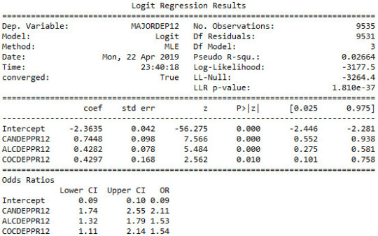
logreg4 = smf.logit(formula = 'MAJORDEP12 ~ CANDEPPR12 + ALCDEPPR12 + COCDEPPR12', data = sub1).fit()

print (logreg4.summary())

# Odd ratios with 95% confidence intervals

print ("Odds Ratios")params = logreg4.paramsconf = logreg4.conf_int()conf['OR'] = paramsconf.columns = ['Lower CI', 'Upper CI', 'OR']

print (numpy.exp(conf))

reult:

[monuonrise]

MULTIPLE REGRESSION MODEL

import numpy

import pandas

import statsmodels.api as sm

import seaborn

import statsmodels.formula.api as smf

import matplotlib.pyplot as plt

# bug fix for display formats to avoid run time errorspandas.set_option('display.float_format', lambda x:'%.2f'%x)nesarc = pandas.read_csv ('nesarc_pds.csv' , low_memory=False)

#Set PANDAS to show all columns in DataFramepandas.set_option('display.max_columns', None)#Set PANDAS to show all rows in DataFramepandas.set_option('display.max_rows', None) nesarc.columns = map(str.upper , nesarc.columns) # Change my variables to numeric nesarc['IDNUM'] =pandas.to_numeric(nesarc['IDNUM'], errors='coerce')nesarc['S3BQ1A5'] = pandas.to_numeric(nesarc['S3BQ1A5'], errors='coerce')nesarc['MAJORDEP12'] = pandas.to_numeric(nesarc['MAJORDEP12'], errors='coerce') # Major depressionnesarc['AGE'] =pandas.to_numeric(nesarc['AGE'], errors='coerce')nesarc['SEX'] = pandas.to_numeric(nesarc['SEX'], errors='coerce')nesarc['S3BD5Q2E'] = pandas.to_numeric(nesarc['S3BD5Q2E'], errors='coerce') # Cannabis use frequencynesarc['S3BQ4'] = pandas.to_numeric(nesarc['S3BQ4'], errors='coerce') # Quantity of joints per daynesarc['GENAXDX12'] = pandas.to_numeric(nesarc['GENAXDX12'], errors='coerce') # General anxietynesarc['S3BD5Q2F'] = pandas.to_numeric(nesarc['S3BD5Q2F'], errors='coerce') # Age when began using cannabis the mostnesarc['DYSDX12'] = pandas.to_numeric(nesarc['DYSDX12'], errors='coerce')

# Dysthymianesarc['SOCPDX12'] = pandas.to_numeric(nesarc['SOCPDX12'], errors='coerce') # Social phobianesarc['S3BD5Q2GR'] = pandas.to_numeric(nesarc['S3BD5Q2GR'], errors='coerce') # Cannabis use duration (weeks)nesarc['S3CD5Q15C'] = pandas.to_numeric(nesarc['S3CD5Q15C'], errors='coerce') # Cannabis dependencenesarc['S3CD5Q13B'] = pandas.to_numeric(nesarc['S3CD5Q13B'], errors='coerce')

# Cannabis abuse # Current cannabis abuse criterianesarc['S3CD5Q14C9'] = pandas.to_numeric(nesarc['S3CD5Q14C9'], errors='coerce')nesarc['S3CQ14A8'] = pandas.to_numeric(nesarc['S3CQ14A8'], errors='coerce') # Longer period cannabis abuse criterianesarc['S3CD5Q14C3'] = pandas.to_numeric(nesarc['S3CD5Q14C3'], errors='coerce') # Depressed because of cannabis effects wearing offnesarc['S3CD5Q14C6C'] = pandas.to_numeric(nesarc['S3CD5Q14C6C'], errors='coerce') # Sleep difficulties because of cannabis effects wearing offnesarc['S3CD5Q14C6R'] = pandas.to_numeric(nesarc['S3CD5Q14C6R'], errors='coerce')

# Eat more because of cannabis effects wearing offnesarc['S3CD5Q14C6H'] = pandas.to_numeric(nesarc['S3CD5Q14C6H'], errors='coerce') # Feel nervous or anxious because of cannabis effects wearing offnesarc['S3CD5Q14C6I'] = pandas.to_numeric(nesarc['S3CD5Q14C6I'], errors='coerce')

# Fast heart beat because of cannabis effects wearing offnesarc['S3CD5Q14C6D'] = pandas.to_numeric(nesarc['S3CD5Q14C6D'], errors='coerce') # Feel weak or tired because of cannabis effects wearing offnesarc['S3CD5Q14C6B'] = pandas.to_numeric(nesarc['S3CD5Q14C6B'], errors='coerce')

# Withdrawal symptomsnesarc['S3CD5Q14C6U'] = pandas.to_numeric(nesarc['S3CD5Q14C6U'], errors='coerce')

# Subset my sample: Cannabis users, ages 18-30 sub1=nesarc[(nesarc['AGE']>=18) & (nesarc['AGE']<=30) & (nesarc['S3BQ1A5']==1)] ###############

Cannabis abuse/dependence criteria in the last 12 months (response variable) ############### #

Current cannabis abuse/dependence criteria #1 DSM-IV def crit1 (row): if row['S3CD5Q14C9']==1 or row['S3CQ14A8'] == 1 : return 1 elif row['S3CD5Q14C9']==2 and row['S3CQ14A8']==2 : return 0sub1['crit1'] = sub1.apply (lambda row: crit1 (row),axis=1) # Current 6 cannabis abuse/dependence sub-symptoms criteria #2 DSM-IV # Recode for summing (from 1,2 to 0,1)recode1 = {1: 1, 2: 0}sub1['S3CD5Q14C6C']=sub1['S3CD5Q14C6C'].replace(9, numpy.nan)sub1['S3CD5Q14C6C']= sub1['S3CD5Q14C6C'].map(recode1)sub1['S3CD5Q14C6R']=sub1['S3CD5Q14C6R'].replace(9, numpy.nan)sub1['S3CD5Q14C6R']= sub1['S3CD5Q14C6R'].map(recode1)sub1['S3CD5Q14C6H']=sub1['S3CD5Q14C6H'].replace(9, numpy.nan)sub1['S3CD5Q14C6H']= sub1['S3CD5Q14C6H'].map(recode1)sub1['S3CD5Q14C6I']=sub1['S3CD5Q14C6I'].replace(9, numpy.nan)sub1['S3CD5Q14C6I']= sub1['S3CD5Q14C6I'].map(recode1)sub1['S3CD5Q14C6D']=sub1['S3CD5Q14C6D'].replace(9, numpy.nan)sub1['S3CD5Q14C6D']= sub1['S3CD5Q14C6D'].map(recode1)sub1['S3CD5Q14C6B']=sub1['S3CD5Q14C6B'].replace(9, numpy.nan)sub1['S3CD5Q14C6B']= sub1['S3CD5Q14C6B'].map(recode1)

# Sum symptomssub1['CWITHDR_COUNT'] = numpy.nansum([sub1['S3CD5Q14C6C'], sub1['S3CD5Q14C6R'], sub1['S3CD5Q14C6H'], sub1['S3CD5Q14C6I'], sub1['S3CD5Q14C6D'], sub1['S3CD5Q14C6B']], axis=0) # Sum code checkchksum=sub1[['IDNUM','S3CD5Q14C6C', 'S3CD5Q14C6R', 'S3CD5Q14C6H', 'S3CD5Q14C6I', 'S3CD5Q14C6D', 'S3CD5Q14C6B', 'CWITHDR_COUNT']]chksum.head(n=50)

# Withdrawal symptoms in the last 12 months (yes/no)def crit2 (row): if row['CWITHDR_COUNT']>=3 or row['S3CD5Q14C6U']==1: return 1 elif row['CWITHDR_COUNT']<3 and row['S3CD5Q14C6U']!=1: return 0sub1['crit2'] = sub1.apply (lambda row: crit2 (row),axis=1) # Longer period cannabis abuse/dependence criteria #3 DSM-IV sub1['S3CD5Q14C3']=sub1['S3CD5Q14C3'].replace(9, numpy.nan)sub1['S3CD5Q14C3']= sub1['S3CD5Q14C3'].map(recode1)

# Current cannabis use cut down criteria #4 DSM-IV sub1['S3CD5Q14C2'] = pandas.to_numeric(sub1['S3CD5Q14C2'], errors='coerce') # Without successsub1['S3CD5Q14C1'] = pandas.to_numeric(sub1['S3CD5Q14C1'], errors='coerce') # More than oncedef crit4 (row): if row['S3CD5Q14C2']==1 or row['S3CD5Q14C1'] == 1 : return 1 elif row['S3CD5Q14C2']==2 and row['S3CD5Q14C1']==2 : return 0sub1['crit4'] = sub1.apply (lambda row: crit4 (row),axis=1)chk1e = sub1['crit4'].value_counts(sort=False, dropna=False)

# Current reduce of important/pleasurable activities criteria #5 DSM-IV sub1['S3CD5Q14C10'] = pandas.to_numeric(sub1['S3CD5Q14C10'], errors='coerce')sub1['S3CD5Q14C11'] = pandas.to_numeric(sub1['S3CD5Q14C11'], errors='coerce')def crit5 (row): if row['S3CD5Q14C10']==1 or row['S3CD5Q14C11'] == 1 : return 1 elif row['S3CD5Q14C10']==2 and row['S3CD5Q14C11']==2 : return 0sub1['crit5'] = sub1.apply (lambda row: crit5 (row),axis=1)chk1g = sub1['crit5'].value_counts(sort=False, dropna=False) # Current cannbis use continuation despite knowledge of physical or psychological problem criteria

#6 DSM-IV sub1['S3CD5Q14C13'] = pandas.to_numeric(sub1['S3CD5Q14C13'], errors='coerce')sub1['S3CD5Q14C12'] = pandas.to_numeric(sub1['S3CD5Q14C12'], errors='coerce')def crit6 (row): if row['S3CD5Q14C13']==1 or row['S3CD5Q14C12'] == 1 : return 1 elif row['S3CD5Q14C13']==2 and row['S3CD5Q14C12']==2 : return 0sub1['crit6'] = sub1.apply (lambda row: crit6 (row),axis=1)chk1h = sub1['crit6'].value_counts(sort=False, dropna=False)

# Cannabis abuse/dependence symptoms sum sub1['CanDepSymptoms'] = numpy.nansum([sub1['crit1'], sub1['crit2'], sub1['S3CD5Q14C3'], sub1['crit4'], sub1['crit5'], sub1['crit6']], axis=0 )chk2 = sub1['CanDepSymptoms'].value_counts(sort=False, dropna=False) ############################################################################### MULTIPLE REGRESSION & CONFIDENCE INTERVALS

############################################################################## sub2 = sub1[['S3BQ4', 'S3BD5Q2F', 'DYSDX12', 'MAJORDEP12', 'CanDepSymptoms', 'SOCPDX12', 'GENAXDX12', 'S3BD5Q2GR']].dropna()

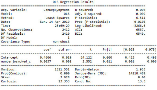
# Centre the quantity of joints smoked per day and age when they began using cannabis, quantitative variablessub1['numberjosmoked_c'] = (sub1['S3BQ4'] - sub1['S3BQ4'].mean())sub1['agebeganuse_c'] = (sub1['S3BD5Q2F'] - sub1['S3BD5Q2F'].mean())sub1['canuseduration_c'] = (sub1['S3BD5Q2GR'] - sub1['S3BD5Q2GR'].mean()) # Linear regression analysis print('OLS regression model for the association between major depression diagnosis and cannabis depndence symptoms')reg1 = smf.ols('CanDepSymptoms ~ MAJORDEP12', data=sub1).fit()print (reg1.summary()) print('OLS regression model for the association of majord depression diagnosis and smoking quantity with cannabis dependence symptoms')reg2 = smf.ols('CanDepSymptoms ~ MAJORDEP12 + DYSDX12', data=sub1).fit()print (reg2.summary()) reg3 = smf.ols('CanDepSymptoms ~ MAJORDEP12 + agebeganuse_c + numberjosmoked_c + canuseduration_c + GENAXDX12 + DYSDX12 + SOCPDX12', data=sub1).fit()print (reg3.summary())

##################################################################################### POLYNOMIAL REGRESSION

#################################################################################### #

First order (linear) scatterplotscat1 = seaborn.regplot(x="S3BQ4", y="CanDepSymptoms", scatter=True, data=sub1)plt.ylim(0, 6)plt.xlabel('Quantity of joints')plt.ylabel('Cannabis dependence symptoms') # Fit second order polynomialscat1 = seaborn.regplot(x="S3BQ4", y="CanDepSymptoms", scatter=True, order=2, data=sub1)plt.ylim(0, 6)plt.xlabel('Quantity of joints')plt.ylabel('Cannabis dependence symptoms') # Linear regression analysisreg4 = smf.ols('CanDepSymptoms ~ numberjosmoked_c', data=sub1).fit()print (reg4.summary()) reg5 = smf.ols('CanDepSymptoms ~ numberjosmoked_c + I(numberjosmoked_c**2)',

data=sub1).fit()print (reg5.summary()) ##################################################################################### EVALUATING MODEL FIT

####################################################################################

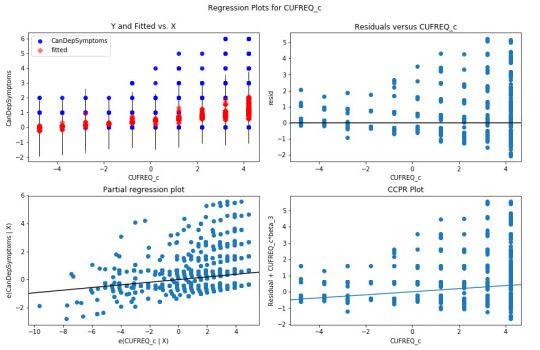
recode1 = {1: 10, 2: 9, 3: 8, 4: 7, 5: 6, 6: 5, 7: 4, 8: 3, 9: 2, 10: 1} # Dictionary with details of frequency variable reverse-recodesub1['CUFREQ'] = sub1['S3BD5Q2E'].map(recode1) # Change variable name from S3BD5Q2E to CUFREQ sub1['CUFREQ_c'] = (sub1['CUFREQ'] - sub1['CUFREQ'].mean()) # Adding frequency of cannabis usereg6 = smf.ols('CanDepSymptoms ~ numberjosmoked_c + I(numberjosmoked_c**2) + CUFREQ_c', data=sub1).fit()print (reg6.summary()) # Q-Q plot for normalityfig1=sm.qqplot(reg6.resid, line='r')print (fig1)

# Simple plot of residualsstdres=pandas.DataFrame(reg6.resid_pearson)fig2=plt.plot(stdres, 'o', ls='None')l = plt.axhline(y=0, color='r')plt.ylabel('Standardized Residual')plt.xlabel('Observation Number') # Additional regression diagnostic plotsfig3 = plt.figure(figsize=(12,8))fig3 = sm.graphics.plot_regress_exog(reg6, "CUFREQ_c", fig=fig3) # leverage plotfig4 = plt.figure(figsize=(36,24))fig4=sm.graphics.influence_plot(reg6, size=2)print(fig4)

OUTPUT:

[monuonrise]

import numpy

import pandas

import statsmodels.formula.api as smf

import statsmodels.stats.multicomp as multi

import seaborn

import matplotlib.pyplot as plt

data = pandas.read_csv('nesarc.csv', low_memory=False)

data['S2DQ1'] = data['S2DQ1'].convert_objects(convert_numeric=True) data['S4AQ7'] = data['S4AQ7'].convert_objects(convert_numeric=True)

data['S2DQ1']=data['S2DQ1'].replace(9, numpy.nan) data['S4AQ7']=data['S4AQ7'].replace(99, numpy.nan) data['S4AQ7']=data['S4AQ7'].replace(' ', numpy.nan) recode1 = {1: 1, 2: 0} data['S2DQ1']= data['S2DQ1'].map(recode1) #centering exp

S4AQ7: NUMBER OF major depression EPISODES

s2dq1: BLOOD/NATURAL FATHER EVER AN ALCOHOLIC OR PROBLEM DRINKER exp

data = data[['S2DQ1', 'S4AQ7']].dropna()

reg1 = smf.ols('S4AQ7 ~ S2DQ1', data=data).fit() print (reg1.summary())

group means & sd

print ("Mean") ds1 = data.groupby('S2DQ1').mean()

print (ds1)

print ("Standard deviation") ds2 = data.groupby('S2DQ1').std()

print (ds2)

[monuonrise]

Regression Modeling in Practice Week 1: Writing About Your Data

Sample

I am using the GapMinder dataset to investigate the relationship between internet usage in a country and that country’s GDP, overall employment rate, female employment rate, and its “polity score”, which is a measure of a country’s democratic and free nature. The sample contains data on a country-level for 215 regions (the 192 U.N. countries, with Serbia and Montenegro aggregated into one, as well as 24 other non-country regions, such as Monaco for instance). The study population is these 215 countries and regions and my sample data is the same; ie, the population is small enough that no sample is necessary to make the data collecting and processing more manageable.

Procedure

The data has been collected by the non-profit venture GapMinder from a handful of sources, including the Institute for Health Metrics and Evaluation, the US Census Bureau’s International Database, the United Nations Statistics Division, and the World Bank. In the case of each data collection organization, data was collected from detailed surveys of the country’s population (such as in a national census) and based mainly upon 2010 data. Employment rate data comes from 2007 and polity score from 2009. Polity score is calculated by subtracting the autocracy score from the democracy score from the Polity IV project’s research. GapMinder’s goal in collecting this data is to help world leaders and their citizens to better understand the forces shaping the geopolitical landscape around the globe.

Measures

My response variable is the internet use rate and my explanatory variables are income per person, employment rate, female employment rate, and polity score. Internet use rate, employment rate, and female employment rate are scaled as percentages of the country’s population. Income per person is simply Gross Domestic Product per capita (the country’s total, country-wide income divided by the population). Polity score is a single measure applied to the whole country. The internet use rate of a country was collected by the World Bank in their World Development Indicators. Income per person is simply the 2010 Gross Domestic Product per capita in constant 2000 USD. The inflation, but not the differences in the cost of living between countries, has been taken into account (this can lead to the seemingly odd case of a having negative income per person, when that country already has very low income relative to the United States plus high inflation, relative to the United States). Both employment rate and female employment rate have been provided by the International Labour Organization. Finally, the polity score has been calculated by the Polity IV project.

I have gone through the data and removed entries where data is missing, when necessary, and sometimes have aggregated data into bins, for histograms, for instance, but otherwise have not modified the data in any way. Deeper data management was unnecessary for the analysis.

[monuonrise]

import pandas

import numpy

import seaborn

import scipy

import matplotlib.pyplot as plt

nesarc = pandas.read_csv ('nesarc_pds.csv', low_memory=False)

Set PANDAS to show all columns in DataFrame

pandas.set_option('display.max_columns' , None)

Set PANDAS to show all rows in DataFrame

pandas.set_option('display.max_rows' , None)

nesarc.columns = map(str.upper , nesarc.columns)

pandas.set_option('display.float_format' , lambda x:'%f'%x)

Change my variables to numeric

nesarc['AGE'] = nesarc['AGE'].convert_objects(convert_numeric=True) nesarc['MAJORDEP12'] = nesarc['MAJORDEP12'].convert_objects(convert_numeric=True) nesarc['S1Q231'] = nesarc['S1Q231'].convert_objects(convert_numeric=True) nesarc['S3BQ1A5'] = nesarc['S3BQ1A5'].convert_objects(convert_numeric=True) nesarc['S3BD5Q2E'] = nesarc['S3BD5Q2E'].convert_objects(convert_numeric=True)

Subset my sample

subset1 = nesarc[(nesarc['AGE']>=18) & (nesarc['AGE']<=30) & nesarc['S3BQ1A5']==1] # Ages 18-30, cannabis users subsetc1 = subset1.copy()

Setting missing data

subsetc1['S1Q231']=subsetc1['S1Q231'].replace(9, numpy.nan) subsetc1['S3BQ1A5']=subsetc1['S3BQ1A5'].replace(9, numpy.nan) subsetc1['S3BD5Q2E']=subsetc1['S3BD5Q2E'].replace(99, numpy.nan) subsetc1['S3BD5Q2E']=subsetc1['S3BD5Q2E'].replace('BL', numpy.nan)

recode1 = {1: 9, 2: 8, 3: 7, 4: 6, 5: 5, 6: 4, 7: 3, 8: 2, 9: 1} # Frequency of cannabis use variable reverse-recode subsetc1['CUFREQ'] = subsetc1['S3BD5Q2E'].map(recode1) # Change the variable name from S3BD5Q2E to CUFREQ

subsetc1['CUFREQ'] = subsetc1['CUFREQ'].astype('category')

Raname graph labels for better interpetation

subsetc1['CUFREQ'] = subsetc1['CUFREQ'].cat.rename_categories(["2 times/year","3-6 times/year","7-11 times/year","Once a month","2-3 times/month","1-2 times/week","3-4 times/week","Nearly every day","Every day"])

Contingency table of observed counts of major depression diagnosis (response variable) within frequency of cannabis use groups (explanatory variable), in ages 18-30

contab1 = pandas.crosstab(subsetc1['MAJORDEP12'], subsetc1['CUFREQ']) print (contab1)

Column percentages

colsum=contab1.sum(axis=0) colpcontab=contab1/colsum print(colpcontab)

Chi-square calculations for major depression within frequency of cannabis use groups

print ('Chi-square value, p value, expected counts, for major depression within cannabis use status') chsq1= scipy.stats.chi2_contingency(contab1) print (chsq1)

Bivariate bar graph for major depression percentages with each cannabis smoking frequency group

plt.figure(figsize=(12,4)) # Change plot size ax1 = seaborn.factorplot(x="CUFREQ", y="MAJORDEP12", data=subsetc1, kind="bar", ci=None) ax1.set_xticklabels(rotation=40, ha="right") # X-axis labels rotation plt.xlabel('Frequency of cannabis use') plt.ylabel('Proportion of Major Depression') plt.show()

recode2 = {1: 10, 2: 9, 3: 8, 4: 7, 5: 6, 6: 5, 7: 4, 8: 3, 9: 2, 10: 1} # Frequency of cannabis use variable reverse-recode subsetc1['CUFREQ2'] = subsetc1['S3BD5Q2E'].map(recode2) # Change the variable name from S3BD5Q2E to CUFREQ2

sub1=subsetc1[(subsetc1['S1Q231']== 1)] sub2=subsetc1[(subsetc1['S1Q231']== 2)]

print ('Association between cannabis use status and major depression for those who lost a family member or a close friend in the last 12 months') contab2=pandas.crosstab(sub1['MAJORDEP12'], sub1['CUFREQ2']) print (contab2)

Column percentages

colsum2=contab2.sum(axis=0) colpcontab2=contab2/colsum2 print(colpcontab2)

Chi-square

print ('Chi-square value, p value, expected counts') chsq2= scipy.stats.chi2_contingency(contab2) print (chsq2)

Line graph for major depression percentages within each frequency group, for those who lost a family member or a close friend

plt.figure(figsize=(12,4)) # Change plot size ax2 = seaborn.factorplot(x="CUFREQ", y="MAJORDEP12", data=sub1, kind="point", ci=None) ax2.set_xticklabels(rotation=40, ha="right") # X-axis labels rotation plt.xlabel('Frequency of cannabis use') plt.ylabel('Proportion of Major Depression') plt.title('Association between cannabis use status and major depression for those who lost a family member or a close friend in the last 12 months') plt.show()

#

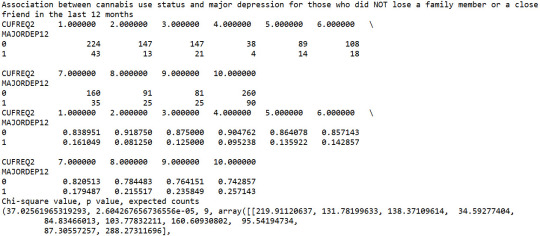
print ('Association between cannabis use status and major depression for those who did NOT lose a family member or a close friend in the last 12 months') contab3=pandas.crosstab(sub2['MAJORDEP12'], sub2['CUFREQ2']) print (contab3)

Column percentages

colsum3=contab3.sum(axis=0) colpcontab3=contab3/colsum3 print(colpcontab3)

Chi-square

print ('Chi-square value, p value, expected counts') chsq3= scipy.stats.chi2_contingency(contab3) print (chsq3)

Line graph for major depression percentages within each frequency group, for those who did NOT lose a family member or a close friend

plt.figure(figsize=(12,4)) # Change plot size ax3 = seaborn.factorplot(x="CUFREQ", y="MAJORDEP12", data=sub2, kind="point", ci=None) ax3.set_xticklabels(rotation=40, ha="right") # X-axis labels rotation plt.xlabel('Frequency of cannabis use') plt.ylabel('Proportion of Major Depression') plt.title('Association between cannabis use status and major depression for those who did NOT lose a family member or a close friend in the last 12 months') plt.show()

[monuonrise]

Generating a Correlation Coefficient

import pandas

import numpy

import seaborn

import scipy

import matplotlib.pyplot as plt

nesarc = pandas.read_csv ('nesarc_pds.csv' , low_memory=False)

Set PANDAS to show all columns in DataFrame

pandas.set_option('display.max_columns', None)

Set PANDAS to show all rows in DataFrame

pandas.set_option('display.max_rows', None)

nesarc.columns = map(str.upper , nesarc.columns)

pandas.set_option('display.float_format' , lambda x:'%f'%x)

Change my variables to numeric

nesarc['AGE'] = pandas.to_numeric(nesarc['AGE'], errors='coerce') nesarc['S3BQ4'] = pandas.to_numeric(nesarc['S3BQ4'], errors='coerce') nesarc['S4AQ6A'] = pandas.to_numeric(nesarc['S4AQ6A'], errors='coerce') nesarc['S3BD5Q2F'] = pandas.to_numeric(nesarc['S3BD5Q2F'], errors='coerce') nesarc['S9Q6A'] = pandas.to_numeric(nesarc['S9Q6A'], errors='coerce') nesarc['S4AQ7'] = pandas.to_numeric(nesarc['S4AQ7'], errors='coerce') nesarc['S3BQ1A5'] = pandas.to_numeric(nesarc['S3BQ1A5'], errors='coerce')

Subset my sample

subset1 = nesarc[(nesarc['S3BQ1A5']==1)] # Cannabis users subsetc1 = subset1.copy()

Setting missing data

subsetc1['S3BQ1A5']=subsetc1['S3BQ1A5'].replace(9, numpy.nan) subsetc1['S3BD5Q2F']=subsetc1['S3BD5Q2F'].replace('BL', numpy.nan) subsetc1['S3BD5Q2F']=subsetc1['S3BD5Q2F'].replace(99, numpy.nan) subsetc1['S4AQ6A']=subsetc1['S4AQ6A'].replace('BL', numpy.nan) subsetc1['S4AQ6A']=subsetc1['S4AQ6A'].replace(99, numpy.nan) subsetc1['S9Q6A']=subsetc1['S9Q6A'].replace('BL', numpy.nan) subsetc1['S9Q6A']=subsetc1['S9Q6A'].replace(99, numpy.nan)

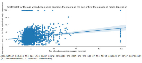
Scatterplot for the age when began using cannabis the most and the age of first episode of major depression

plt.figure(figsize=(12,4)) # Change plot size scat1 = seaborn.regplot(x="S3BD5Q2F", y="S4AQ6A", fit_reg=True, data=subset1) plt.xlabel('Age when began using cannabis the most') plt.ylabel('Age when expirenced the first episode of major depression') plt.title('Scatterplot for the age when began using cannabis the most and the age of first the episode of major depression') plt.show()

data_clean=subset1.dropna()

Pearson correlation coefficient for the age when began using cannabis the most and the age of first the episode of major depression

print ('Association between the age when began using cannabis the most and the age of the first episode of major depression') print (scipy.stats.pearsonr(data_clean['S3BD5Q2F'], data_clean['S4AQ6A']))

Scatterplot for the age when began using cannabis the most and the age of the first episode of general anxiety

plt.figure(figsize=(12,4)) # Change plot size scat2 = seaborn.regplot(x="S3BD5Q2F", y="S9Q6A", fit_reg=True, data=subset1) plt.xlabel('Age when began using cannabis the most') plt.ylabel('Age when expirenced the first episode of general anxiety') plt.title('Scatterplot for the age when began using cannabis the most and the age of the first episode of general anxiety') plt.show()

Pearson correlation coefficient for the age when began using cannabis the most and the age of the first episode of general anxiety

print ('Association between the age when began using cannabis the most and the age of first the episode of general anxiety') print (scipy.stats.pearsonr(data_clean['S3BD5Q2F'], data_clean['S9Q6A']))

This assignment aims to statistically assess the evidence, provided by NESARC codebook, in favor of or against the association between cannabis use and mental illnesses, such as major depression and general anxiety, in U.S. adults. More specifically, since my research question includes only categorical variables, I selected three new quantitative variables from the NESARC codebook. Therefore, I redefined my hypothesis and examined the correlation between the age when the individuals began using cannabis the most (quantitative explanatory, variable“S3BD5Q2F”) and the age when they experienced the first episode of major depression and general anxiety (quantitative response, variables“S4AQ6A”and”S9Q6A”). As a result, in the first place, in order to visualize the association between cannabis use and both depression and anxiety episodes, I used seaborn library to produce a scatterplot for each disorder separately and interpreted the overall patterns, by describing the direction, as well as the form and the strength of the relationships. In addition, I ran Pearson correlation test (Q->Q) twice (once for each disorder) and measured the strength of the relationships between each pair of quantitative variables, by numerically generating both the correlation coefficients r and the associated p-values. For the code and the output I used Spyder (IDE).

The three quantitative variables that I used for my Pearson correlation tests are:

[monuonrise]

import pandas

import numpy

import scipy.stats

import seaborn

import matplotlib.pyplot as plt

nesarc = pandas.read_csv ('nesarc_pds.csv' , low_memory=False)

Set PANDAS to show all columns in DataFrame

pandas.set_option('display.max_columns', None)

#Set PANDAS to show all rows in DataFrame

pandas.set_option('display.max_rows', None)

nesarc.columns = map(str.upper , nesarc.columns)

pandas.set_option('display.float_format' , lambda x:'%f'%x)

#Change my variables to numeric

nesarc['AGE'] = pandas.to_numeric(nesarc['AGE'], errors='coerce') nesarc['S3BQ4'] = pandas.to_numeric(nesarc['S3BQ4'], errors='coerce') nesarc['S3BQ1A5'] = pandas.to_numeric(nesarc['S3BQ1A5'], errors='coerce') nesarc['S3BD5Q2B'] = pandas.to_numeric(nesarc['S3BD5Q2B'], errors='coerce') nesarc['S3BD5Q2E'] = pandas.to_numeric(nesarc['S3BD5Q2E'], errors='coerce') nesarc['MAJORDEP12'] = pandas.to_numeric(nesarc['MAJORDEP12'], errors='coerce') nesarc['GENAXDX12'] = pandas.to_numeric(nesarc['GENAXDX12'], errors='coerce')

#Subset my sample

subset1 = nesarc[(nesarc['AGE']>=18) & (nesarc['AGE']<=30)] # Ages 18-30 subsetc1 = subset1.copy()

subset2 = nesarc[(nesarc['AGE']>=18) & (nesarc['AGE']<=30) & (nesarc['S3BQ1A5']==1)] # Cannabis users, ages 18-30 subsetc2 = subset2.copy()

#Setting missing data for frequency and cannabis use, variables S3BD5Q2E, S3BQ1A5

subsetc1['S3BQ1A5']=subsetc1['S3BQ1A5'].replace(9, numpy.nan) subsetc2['S3BD5Q2E']=subsetc2['S3BD5Q2E'].replace('BL', numpy.nan) subsetc2['S3BD5Q2E']=subsetc2['S3BD5Q2E'].replace(99, numpy.nan)

Contingency table of observed counts of major depression diagnosis (response variable) within cannabis use (explanatory variable), in ages 18-30

contab1=pandas.crosstab(subsetc1['MAJORDEP12'], subsetc1['S3BQ1A5']) print (contab1)

#Column percentages

colsum=contab1.sum(axis=0) colpcontab=contab1/colsum print(colpcontab)

#Chi-square calculations for major depression within cannabis use status

print ('Chi-square value, p value, expected counts, for major depression within cannabis use status') chsq1= scipy.stats.chi2_contingency(contab1) print (chsq1)

#Contingency table of observed counts of geberal anxiety diagnosis (response variable) within cannabis use (explanatory variable), in ages 18-30

contab2=pandas.crosstab(subsetc1['GENAXDX12'], subsetc1['S3BQ1A5']) print (contab2)

#Column percentages

colsum2=contab2.sum(axis=0) colpcontab2=contab2/colsum2 print(colpcontab2)

#Chi-square calculations for general anxiety within cannabis use status

print ('Chi-square value, p value, expected counts, for general anxiety within cannabis use status') chsq2= scipy.stats.chi2_contingency(contab2) print (chsq2)

#

#Contingency table of observed counts of major depression diagnosis (response variable) within frequency of cannabis use (10 level explanatory variable), in ages 18-30

contab3=pandas.crosstab(subset2['MAJORDEP12'], subset2['S3BD5Q2E']) print (contab3)

#Column percentages

colsum3=contab3.sum(axis=0) colpcontab3=contab3/colsum3 print(colpcontab3)

#Chi-square calculations for mahor depression within frequency of cannabis use groups

print ('Chi-square value, p value, expected counts for major depression associated frequency of cannabis use') chsq3= scipy.stats.chi2_contingency(contab3) print (chsq3)

recode1 = {1: 9, 2: 8, 3: 7, 4: 6, 5: 5, 6: 4, 7: 3, 8: 2, 9: 1} # Dictionary with details of frequency variable reverse-recode subsetc2['CUFREQ'] = subsetc2['S3BD5Q2E'].map(recode1) # Change variable name from S3BD5Q2E to CUFREQ

subsetc2["CUFREQ"] = subsetc2["CUFREQ"].astype('category')

#Rename graph labels for better interpretation

subsetc2['CUFREQ'] = subsetc2['CUFREQ'].cat.rename_categories(["2 times/year","3-6 times/year","7-11 times/years","Once a month","2-3 times/month","1-2 times/week","3-4 times/week","Nearly every day","Every day"])

#Graph percentages of major depression within each cannabis smoking frequency group

plt.figure(figsize=(12,4)) # Change plot size ax1 = seaborn.factorplot(x="CUFREQ", y="MAJORDEP12", data=subsetc2, kind="bar", ci=None) ax1.set_xticklabels(rotation=40, ha="right") # X-axis labels rotation plt.xlabel('Frequency of cannabis use') plt.ylabel('Proportion of Major Depression') plt.show()

#Post hoc test, pair comparison of frequency groups 1 and 9, 'Every day' and '2 times a year'

recode2 = {1: 1, 9: 9} subsetc2['COMP1v9']= subsetc2['S3BD5Q2E'].map(recode2)

#Contingency table of observed counts

ct4=pandas.crosstab(subsetc2['MAJORDEP12'], subsetc2['COMP1v9']) print (ct4)

#Column percentages

colsum4=ct4.sum(axis=0) colpcontab4=ct4/colsum4 print(colpcontab4)

#Chi-square calculations for pair comparison of frequency groups 1 and 9, 'Every day' and '2 times a year'

print ('Chi-square value, p value, expected counts, for pair comparison of frequency groups -Every day- and -2 times a year-') cs4= scipy.stats.chi2_contingency(ct4) print (cs4)

#Post hoc test, pair comparison of frequency groups 2 and 6, 'Nearly every day' and 'Once a month'

recode3 = {2: 2, 6: 6} subsetc2['COMP2v6']= subsetc2['S3BD5Q2E'].map(recode3)

#Contingency table of observed counts

ct5=pandas.crosstab(subsetc2['MAJORDEP12'], subsetc2['COMP2v6']) print (ct5)

#Column percentages

colsum5=ct5.sum(axis=0) colpcontab5=ct5/colsum5 print(colpcontab5)

#Chi-square calculations for pair comparison of frequency groups 2 and 6, 'Nearly every day' and 'Once a month'

print ('Chi-square value, p value, expected counts for pair comparison of frequency groups -Nearly every day- and -Once a month-') cs5= scipy.stats.chi2_contingency(ct5) print (cs5)

[monuonrise]

Analysis of Variance

Analysis of Variance Below is the code to make the ANOVA technique:

First I have imported the libraries and management the data like in the other assignments presented until here.

import pandas import numpy import statistics import statsmodels.formula.api as smf import statsmodels.stats.multicomp as multi

Import the data set to memory

data = pandas.read_csv("separatedData.csv", low_memory = False)

Change data type among variables to numeric

data["breastCancer100th"] = data["breastCancer100th"].convert_objects(convert_numeric=True) data["meanSugarPerson"] = data["meanSugarPerson"].convert_objects(convert_numeric=True)

Create a subData with only the variables breastCancer100th, meanSugarPerson, meanFoodPerson, meanCholesterol

sub1=data[['breastCancer100th', 'meanSugarPerson']]

Create the conditions to a new variable named sugar_consumption that will categorize the meanSugarPerson answers

def sugar_consumption (row): if 0 < row['meanSugarPerson'] <= 30 : return 0 # Desirable between 0 and 30 g. if 30 < row['meanSugarPerson'] <= 60 : return 1 # Raised between 30 and 60 g. if 60 < row['meanSugarPerson'] <= 90 : return 2 # Borderline high between 60 and 90 g. if 90 < row['meanSugarPerson'] <= 120 : return 3 # High between 90 and 120 g. if row['meanSugarPerson'] > 120 : return 4 # Very high under 120g.

Add the new variable sugar_consumption to subData

sub1['sugar_consumption'] = sub1.apply (lambda row: sugar_consumption (row),axis=1) Then I have created a new sub data and make the ANOVA method.

creating a sub data with only the breast cancer cases and the sugar consumption mean

sub2 = sub1[['breastCancer100th', 'sugar_consumption']].dropna()

using ols function for calculating the F-statistic and associated p value

model1 = smf.ols(formula='breastCancer100th ~ C(sugar_consumption)', data=sub2).fit() print (model1.summary())

OLS Regression Results

Dep. Variable: breastCancer100th R-squared: 0.411 Model: OLS Adj. R-squared: 0.392 Method: Least Squares F-statistic: 21.59 Date: Fri, 29 Jul 2016 Prob (F-statistic): 1.55e-13 Time: 19:03:11 Log-Likelihood: -560.14 No. Observations: 129 AIC: 1130. Df Residuals: 124 BIC: 1145. Df Model: 4

Covariance Type: nonrobust

coef std err t P>|t| [95.0% Conf. Int.]

Intercept 20.6481 3.651 5.655 0.000 13.421 27.875 C(sugar_consumption)[T.1] 2.9940 5.682 0.527 0.599 -8.251 14.239 C(sugar_consumption)[T.2] 14.0744 4.995 2.818 0.006 4.189 23.960 C(sugar_consumption)[T.3] 25.3777 4.995 5.081 0.000 15.492 35.263

C(sugar_consumption)[T.4] 45.5661 5.520 8.254 0.000 34.640 56.493

Omnibus: 2.575 Durbin-Watson: 1.688 Prob(Omnibus): 0.276 Jarque-Bera (JB): 2.533 Skew: 0.336 Prob(JB): 0.282

Kurtosis: 2.864 Cond. No. 5.76

Warnings: [1] Standard Errors assume that the covariance matrix of the errors is correctly specified. We can see that the F-test is 21.59 and the p-value is lower than 0.05 indicating that the null hypothesis is false.

For the mean and the standard deviation we have:

means for breast cancer by sugar consumption

print ('means for breast cancer by sugar consumption') m1= sub2.groupby('sugar_consumption').mean() print (m1)

standard deviations for breast cancer by sugar consumption

print ('standard deviations for breast cancer by sugar consumption') sd1 = sub2.groupby('sugar_consumption').std() print (sd1) means for breast cancer by sugar consumption

sugar_consumption breastCancer100th 0 20.648148 1 23.642105 2 34.722581 3 46.025806 4 66.214286

standard deviations for breast cancer by sugar consumption

sugar_consumption breastCancer100th 0 6.607535 1 10.970228 2 16.280432 3 26.222649 4 25.255302 We can see that the mean for each category is different but there are some categories that have a close value. However, as we have five categories in the explanatory variable, we need to make a Post hoc test in order to avoid the type 1 error.

Post hoc test

Post hoc test for ANOVA (as the categorical variable have five categories)

mc1 = multi.MultiComparison(sub2['breastCancer100th'], sub2['sugar_consumption']) res1 = mc1.tukeyhsd() print(res1.summary())

Multiple Comparison of Means - Tukey HSD,FWER=0.05

group1 group2 meandiff lower upper reject

0 1 2.994 -12.7348 18.7227 False 0 2 14.0744 0.2475 27.9013 True 0 3 25.3777 11.5508 39.2045 True 0 4 45.5661 30.2834 60.8489 True 1 2 11.0805 -4.2234 26.3843 False 1 3 22.3837 7.0799 37.6875 True 1 4 42.5722 25.9412 59.2031 True 2 3 11.3032 -2.0384 24.6448 False 2 4 31.4917 16.6466 46.3368 True

3 4 20.1885 5.3433 35.0336 True

The Post hoc test presented us that only three comparison groups have the null hypothesis confirmed. The groups are:

(0) Desirable with (1) Raised (1) Raised with (2) Borderline high (2) Borderline high with (3) High This means that the amount of new breast cancer cases among the population that intakes sugar in the proportions of this groups doesn’t have a significant difference. However, to the other seven comparisons, the post hoc test presents that the null hypothesis is false, demonstrating that the high consumption of sugar has a relation with a greater incidence of breast cancer case.

Analysis of Variance Below is the code to make the ANOVA technique:

First I have imported the libraries and management the data like in the other assignments presented until here.

import pandas import numpy import statistics import statsmodels.formula.api as smf import statsmodels.stats.multicomp as multi

Import the data set to memory

data = pandas.read_csv("separatedData.csv", low_memory = False)

Change data type among variables to numeric

data["breastCancer100th"] = data["breastCancer100th"].convert_objects(convert_numeric=True) data["meanSugarPerson"] = data["meanSugarPerson"].convert_objects(convert_numeric=True)

Create a subData with only the variables breastCancer100th, meanSugarPerson, meanFoodPerson, meanCholesterol

sub1=data[['breastCancer100th', 'meanSugarPerson']]

Create the conditions to a new variable named sugar_consumption that will categorize the meanSugarPerson answers

def sugar_consumption (row): if 0 < row['meanSugarPerson'] <= 30 : return 0 # Desirable between 0 and 30 g. if 30 < row['meanSugarPerson'] <= 60 : return 1 # Raised between 30 and 60 g. if 60 < row['meanSugarPerson'] <= 90 : return 2 # Borderline high between 60 and 90 g. if 90 < row['meanSugarPerson'] <= 120 : return 3 # High between 90 and 120 g. if row['meanSugarPerson'] > 120 : return 4 # Very high under 120g.

Add the new variable sugar_consumption to subData

sub1['sugar_consumption'] = sub1.apply (lambda row: sugar_consumption (row),axis=1) Then I have created a new sub data and make the ANOVA method.

creating a sub data with only the breast cancer cases and the sugar consumption mean

sub2 = sub1[['breastCancer100th', 'sugar_consumption']].dropna()

using ols function for calculating the F-statistic and associated p value

model1 = smf.ols(formula='breastCancer100th ~ C(sugar_consumption)', data=sub2).fit() print (model1.summary())

OLS Regression Results

Dep. Variable: breastCancer100th R-squared: 0.411 Model: OLS Adj. R-squared: 0.392 Method: Least Squares F-statistic: 21.59 Date: Fri, 29 Jul 2016 Prob (F-statistic): 1.55e-13 Time: 19:03:11 Log-Likelihood: -560.14 No. Observations: 129 AIC: 1130. Df Residuals: 124 BIC: 1145. Df Model: 4

Covariance Type: nonrobust

coef std err t P>|t| [95.0% Conf. Int.]

Intercept 20.6481 3.651 5.655 0.000 13.421 27.875 C(sugar_consumption)[T.1] 2.9940 5.682 0.527 0.599 -8.251 14.239 C(sugar_consumption)[T.2] 14.0744 4.995 2.818 0.006 4.189 23.960 C(sugar_consumption)[T.3] 25.3777 4.995 5.081 0.000 15.492 35.263

C(sugar_consumption)[T.4] 45.5661 5.520 8.254 0.000 34.640 56.493

Omnibus: 2.575 Durbin-Watson: 1.688 Prob(Omnibus): 0.276 Jarque-Bera (JB): 2.533 Skew: 0.336 Prob(JB): 0.282

Kurtosis: 2.864 Cond. No. 5.76

Warnings: [1] Standard Errors assume that the covariance matrix of the errors is correctly specified. We can see that the F-test is 21.59 and the p-value is lower than 0.05 indicating that the null hypothesis is false.

For the mean and the standard deviation we have:

means for breast cancer by sugar consumption

print ('means for breast cancer by sugar consumption') m1= sub2.groupby('sugar_consumption').mean() print (m1)

standard deviations for breast cancer by sugar consumption

print ('standard deviations for breast cancer by sugar consumption') sd1 = sub2.groupby('sugar_consumption').std() print (sd1) means for breast cancer by sugar consumption

sugar_consumption breastCancer100th 0 20.648148 1 23.642105 2 34.722581 3 46.025806 4 66.214286

standard deviations for breast cancer by sugar consumption

sugar_consumption breastCancer100th 0 6.607535 1 10.970228 2 16.280432 3 26.222649 4 25.255302 We can see that the mean for each category is different but there are some categories that have a close value. However, as we have five categories in the explanatory variable, we need to make a Post hoc test in order to avoid the type 1 error.

Post hoc test

Post hoc test for ANOVA (as the categorical variable have five categories)

mc1 = multi.MultiComparison(sub2['breastCancer100th'], sub2['sugar_consumption']) res1 = mc1.tukeyhsd() print(res1.summary())

Multiple Comparison of Means - Tukey HSD,FWER=0.05

group1 group2 meandiff lower upper reject

0 1 2.994 -12.7348 18.7227 False 0 2 14.0744 0.2475 27.9013 True 0 3 25.3777 11.5508 39.2045 True 0 4 45.5661 30.2834 60.8489 True 1 2 11.0805 -4.2234 26.3843 False 1 3 22.3837 7.0799 37.6875 True 1 4 42.5722 25.9412 59.2031 True 2 3 11.3032 -2.0384 24.6448 False 2 4 31.4917 16.6466 46.3368 True

3 4 20.1885 5.3433 35.0336 True

The Post hoc test presented us that only three comparison groups have the null hypothesis confirmed. The groups are:

(0) Desirable with (1) Raised (1) Raised with (2) Borderline high (2) Borderline high with (3) High This means that the amount of new breast cancer cases among the population that intakes sugar in the proportions of this groups doesn’t have a significant difference. However, to the other seven comparisons, the post hoc test presents that the null hypothesis is false, demonstrating that the high consumption of sugar has a relation with a greater incidence of breast cancer case.

[monuonrise]

Final Analysis on my Research

So guys the work has come to an end. in this post I am going to show you the relations between the data variables I took and their dependencies on each other.

So here we first start the code by showing uni variate graphs for all variables.

Then we will see all the bi variate graphs and then comes the relationship between them into the scene.

We analyze the graphs of the relationship between the variables in two ways . They are:

The relationship between co2 emission and urban rate

The relationship between co2 emission and life expectancy rate

The first one will describe how the co2 is growing due to urban population

The second relation describes the effect of co2 on life expectancy rate

The code for the program is as shown below. You can refer the comments for clarity.

The output for above code is as shown below

Note: For graphs I have considered all values in x and y axis to get an over all view . So the last graphs will have different colors showing the relation on overall data

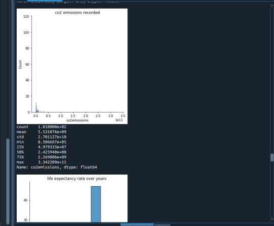
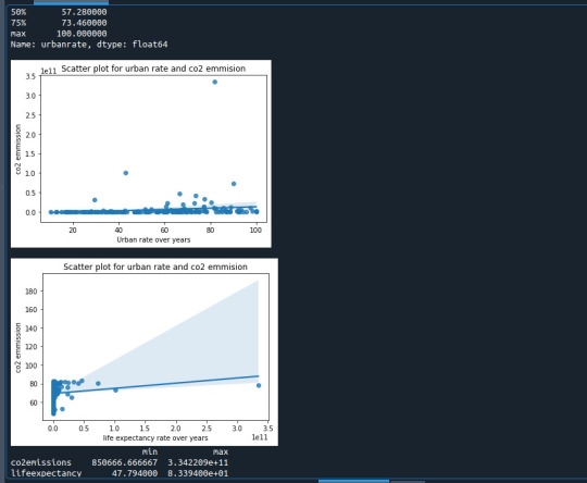
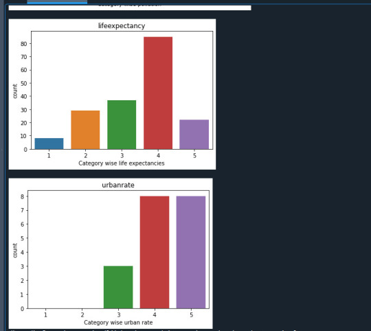
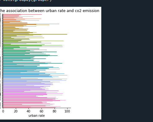
I apologies for the length of outputs !!

RESULT:

In the graphs in outputs seen above we can conclude our outputs;

1.As the urban rate increased we see that there is an increase in co2 emission in the environment. We can even see this in our world that as the population is growing the pollution i.e; co2 emission is also growing

2.And as the pollution is growing the life expectancy rate is also decreasing. The oxygen levels are decreasing due to more carbon dioxide emission which is severely decreasing the life expectancy rate.

So guys in final I conclude that increase in co2 emission is reducing the life expectancy rate for ever year.

And here my research Ends......

[monuonrise]

Making Data Management Decisions on my Work

It is very important to set the data properly before we start analysis on our project.

The first step we take here is set the data into numeric type.

Then we will remove null values from the information gathered .

Then we will group data by setting boundaries on own.

The below code shows the work performed on my data. There comments in code to help you understand each step in it.

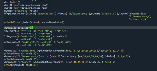
The outputs for above code is as shown below:

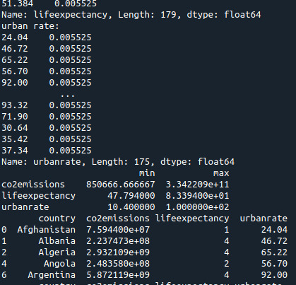
Here we notice that we removed all the null values. Grouped the data using our boundaries and we displayed their absolute and relative frequencies. So in this way we preprocess our data before analyzing it.

[monuonrise]

Frequency report on my Project

My Program for getting frequencies of my data set is proceeded as below

The number of rows and columns are:

And the frequencies values are as shown below:

1.Frequency for co2 emission:

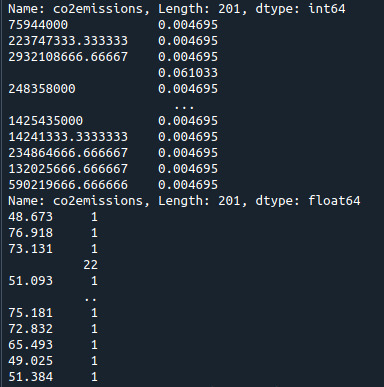
2.Frequency for life expectancy and urban rate:

3. For group by data:

Above are the values which were resulted from the code. It represents the frequency of different variables. And in my program the resulted frequency values are for co2 emission, life expectancy and for urban rate.

My data doesn't have any categorical data so I am not showing any relational analysis in the above code..

That's it for the week Guys!!!!!!

[monuonrise]

MY RESEARCH PROJECT

Hi guys!!!!

I am very glad to say that I am starting my new Research Project. My project is based on the effects of co2 emission on breast cancer. So basically, I am going to use the datasets from gap minder. I even studied a journal named The Relationships between CO2 Emissions; Breast cancer related to my research area. The reason for me to select this area is the amount of CO2 being produced. Guys you might be knowing that in earlier days as there were no industries from years breast cancer is a problem among most of the Women's. As the era change Women's started working in many technological fields. This project deals with the contribution of CO2 on Women's.

I hope my research will be successful!!!