sarahayton

[sarahayton]

Running a k-means Cluster Analysis

A k-means cluster analysis was conducted to identify subgroups of people based on their similarity across 16 variables that might have an impact on marijuana use. Clustering variables included a number of characteristics including: age, alcohol and other substance use (ALCEVR1, ALCPROBS1, COCEVER1, INHEVER1), behavioral (DEP1, ESTEEM1, VIOL1), as well as educational (DEVIANT1, GPA1, EXPEL1) and family (FAMCONCT, PARACTV, PARPRES) characteristics. All predictors were standardized to have a mean value of zero and a standard deviation of one.

data = pd.read_csv("tree_addhealth.csv")

cluster=data_clean[['AGE', 'ALCEVR1', 'ALCPROBS1', 'COCEVER1', 'INHEVER1', 'CIGAVAIL', 'DEP1', 'ESTEEM1', 'VIOL1', 'PASSIST', 'DEVIANT1', 'GPA1', 'EXPEL1', 'FAMCONCT','PARACTV', 'PARPRES']]

Data were randomly split into a training set that included 70% of the observationsand a test set that included 30% of the observations. A series of k-means cluster analyses were conducted on the training data specifying k=1-9 clusters, using Euclidean distance. The variance in the clustering variables that was accounted for by the clusters (r-square) was plotted for each of the nine cluster solutions in an elbow curve to provide guidance for choosing the number of clusters to interpret.

clus_train, clus_test = train_test_split(clustervar, test_size=.3, random_state=123)

from scipy.spatial.distance import cdist

clusters=range(1,10)

meandist=[]

for k in clusters:

model=KMeans(n_clusters=k)

model.fit(clus_train)

clusassign=model.predict(clus_train)

meandist.append(sum(np.min(cdist(clus_train, model.cluster_centers_, 'euclidean'), axis=1)) / clus_train.shape[0])

plt.plot(clusters, meandist)

plt.xlabel('Number of clusters')

plt.ylabel('Average distance')

plt.title('Selecting k with the Elbow Method')

Figure 1. Elbow curve of r-square values for the nine cluster solutions

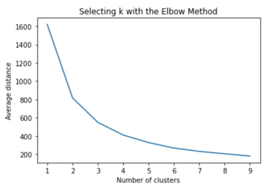
The elbow curve was inconclusive, suggesting that the 2 and 3-cluster solutions might be interpreted. The results below are for an interpretation of the 3-cluster solution.

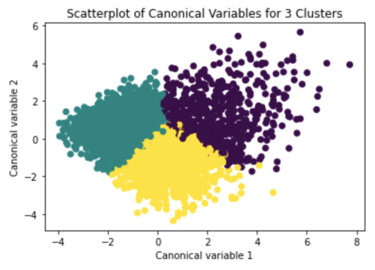
Canonical discriminant analyses was used to reduce the 16 clustering variable down a few variables that accounted for most of the variance in the clustering variables. A scatterplot of the first two canonical variables by cluster (Figure 2 shown below) indicated that the observations in clusters 1 and 4 were densely packed with relatively low within cluster variance, and did not overlap very much with the other clusters. Cluster 2 was generally distinct, but the observations had greater spread suggesting higher within cluster variance. Observations in cluster 3 were spread out more than the other clusters, showing high within cluster variance. The results of this plot suggest that the best cluster solution may have fewer than 4 clusters, so it will be especially important to also evaluate the cluster solutions with fewer than 4 clusters.

model3=KMeans(n_clusters=3)

model3.fit(clus_train)

clusassign=model3.predict(clus_train)

pca_2 = PCA(2)

Figure 2. Plot of the first two canonical variables for the clustering variables by cluster.

clustergrp = merged_train.groupby('cluster').mean()

print ("Clustering variable means by cluster")

print(clustergrp)

Clustering variable means by cluster

cluster

AGE ALCEVR1 ALCPROBS1 COCEVER1 \

0 17.007748 0.685719 0.981627 0.109325

1 15.053934 -0.448153 -0.340980 0.008289

2 17.758390 0.129689 -0.161056 0.015962

INHEVER1 CIGAVAIL DEP1 ESTEEM1 VIOL1 PASSIST DEVIANT1 \

0 0.180064 0.446945 0.849564 -0.660382 0.830998 0.146302 1.178689

1 0.039940 0.229088 -0.310095 0.244037 -0.170265 0.092690 -0.366272

2 0.039106 0.292897 -0.139679 0.118059 -0.254260 0.091780 -0.220419

GPA1 EXPEL1 FAMCONCT PARACTV PARPRES

0 2.401125 0.098071 -1.096106 -0.439664 -0.563944

1 2.997048 0.017332 0.329184 0.114663 0.149519

2 2.835129 0.031923 0.220210 0.113718 0.132120

The means on the clustering variables showed that, compared to the other clusters, those in cluster 1 had the highest levels of alcohol use, alcohol problems, cocaine use, cigarette access and smoking, depression, violence, deviant behavior, and expulsion. This cluster also had the lowest self esteem, GPA, family connectedness, and parental presence. Those in cluster 2 were younger and had the lowest levels of prior alcohol or substance use, lowest levels of depression and expulsion, and the highest levels of self esteem and GPA. Those in cluster 3 clearly were the oldest and least violent, and fell between clusters 1 and 2 in all other characteristics.

m1= sub1.groupby('cluster').mean()

MAREVER1 cluster

0 0.612540

1 0.086662

2 0.223464

gpamod = smf.ols(formula='MAREVER1 ~ C(cluster)', data=sub1).fit()

mc1 = multi.MultiComparison(sub1['MAREVER1'], sub1['cluster'])

res1 = mc1.tukeyhsd()

Multiple Comparison of Means - Tukey HSD, FWER=0.05 =================================================== group1 group2 meandiff p-adj lower upper reject

---------------------------------------------------

0 1 -0.5259 0.001 -0.5696 -0.4822 True

0 2 -0.3891 0.001 -0.4332 -0.345 True

1 2 0.1368 0.001 0.1014 0.1722 True

---------------------------------------------------

In order to externally validate the clusters, an Analysis of Variance (ANOVA) was conducting to test for significant differences between the clusters on marijuana use. A tukey test was used for post hoc comparisons between the clusters. The tukey post hoc comparisons showed significant differences between all clusters on marijuana use (all p < 0.001). Those in cluster 1 had the highest marijuana use (mean=0.6125, sd=0.4876), and cluster 2 had the lowest marijuana use (mean=0.0866, sd=0.2814).

[sarahayton]

Running a Lasso Regression Analysis

A lasso regression analysis was conducted to identify a subset of variables from a pool of 22 predictor variables that best predicted a marijuana use. Predictors included number of characteristics including the following which were estimated to have non-zero coefficients: race and ethnicity (WHITE and BLACK), age, alcohol and other substance use (ALCEVR1, ALCPROBS1, COCEVER1, INHEVER1), as well as educational (DEVIANT1, GPA1, EXPEL1) characteristics. All predictors were standardized to have a mean value of zero and a standard deviation of one.

data = pd.read_csv("tree_addhealth.csv")

predvar = data_clean[['MALE', 'HISPANIC', 'WHITE', 'BLACK', 'NAMERICAN', 'ASIAN', 'AGE', 'ALCEVR1', 'ALCPROBS1', 'COCEVER1', 'INHEVER1', 'CIGAVAIL', 'DEP1', 'ESTEEM1', 'VIOL1', 'PASSIST', 'DEVIANT1', 'GPA1', 'EXPEL1', 'FAMCONCT', 'PARACTV', 'PARPRES']]

target = data_clean.MAREVER1

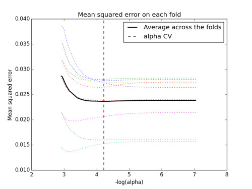
Data were randomly split into a training set that included 70% of the observations (N=3201) and a test set that included 30% of the observations (N=1701). The least angle regression algorithm with k=10 fold cross validation was used to estimate the lasso regression model in the training set, and the model was validated using the test set. The change in the cross validation average (mean) squared error at each step was used to identify the best subset of predictor variables.

pred_train, pred_test, tar_train, tar_test = train_test_split(predictors, target, test_size=.3, random_state=123)

model = LassoLarsCV(cv=10, precompute=False).fit(pred_train,tar_train)

Figure 1. Change in the validation MSE at each step

m_log_alphascv = -np.log10(model.cv_alphas_)

plt.figure()

plt.plot(m_log_alphascv, model.cv_mse_path_, ':')

plt.plot(m_log_alphascv, model.cv_mse_path_.mean(axis=-1), 'k',

label='Average across the folds', linewidth=2)

plt.axvline(-np.log10(model.alpha_), linestyle='--', color='k',

label='alpha CV')

plt.legend()

plt.xlabel('-log(alpha)')

plt.ylabel('Mean squared error')

plt.title('Mean squared error on each fold')

Of the 22 predictor variables, 10 were retained in the selected model. During the estimation process, alcohol use and problems were most strongly associated with marijuana use, followed by cocaine use and GPA. Alcohol and cocaine characteristics were positively associated with marijuana use, while GPA was negatively associated with marijuana use. These 10 variables accounted for 32.8% of the variance in marijuana use in the test set.

[sarahayton]

Running a Random Forest

Random forest analysis was performed to evaluate the importance of a series of explanatory variables in predicting a binary, categorical response variable. Demographic explanatory variables were included as possible contributors to a random forest evaluating regular smoking (my response variable).

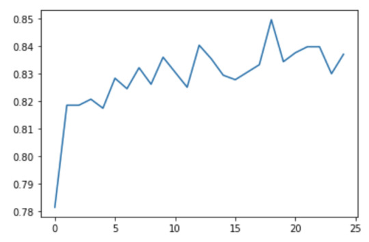
We can examine variable importances, and see that the 10th variable, marever1 has the highest importance (0.11357189). The accuracy of the random forest was about 83%. We can also see that the accuracy of our random forest appears to increase with the growing number of trees.

Load the dataset

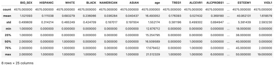
AH_data = pd.read_csv("tree_addhealth.csv") data_clean = AH_data.dropna() data_clean.dtypes data_clean.describe()

Split into training and testing sets

predictors = data_clean[['BIO_SEX','HISPANIC','WHITE','BLACK','NAMERICAN','ASIAN','age', 'ALCEVR1','ALCPROBS1','marever1','cocever1','inhever1','cigavail','DEP1','ESTEEM1','VIOL1', 'PASSIST','DEVIANT1','SCHCONN1','GPA1','EXPEL1','FAMCONCT','PARACTV','PARPRES']] targets = data_clean.TREG1 pred_train, pred_test, tar_train, tar_test  = train_test_split(predictors, targets, test_size=.4) print (pred_train.shape) print (pred_test.shape) print (tar_train.shape) print (tar_test.shape)

Build model on the training data

from sklearn.ensemble import RandomForestClassifier

classifier=RandomForestClassifier(n_estimators=25)

classifier=classifier.fit(pred_train,tar_train)

predictions=classifier.predict(pred_test)

sklearn.metrics.confusion_matrix(tar_test,predictions)

sklearn.metrics.accuracy_score(tar_test, predictions)

> 0.8316939890710382

model = ExtraTreesClassifier()

model.fit(pred_train,tar_train)

# display the relative importance of each attribute

print(model.feature_importances_)

>[0.02766765 0.01413192 0.02233968 0.01849067 0.0068074 0.00702528 0.06190131 0.04751572 0.05191577 0.11357189 0.01404674 0.0162488 0.02871579 0.06181769 0.05610384 0.05358636 0.01844548 0.06395176 0.06465236 0.0707823 0.01252415 0.05998488 0.05762042 0.05015213]

trees=range(25)

accuracy=np.zeros(25)

for idx in range(len(trees)):

classifier=RandomForestClassifier(n_estimators=idx + 1)

classifier=classifier.fit(pred_train,tar_train)

predictions=classifier.predict(pred_test)

accuracy[idx]=sklearn.metrics.accuracy_score(tar_test, predictions)

plt.cla()

plt.plot(trees, accuracy)

[sarahayton]

Classification Tree

Here I used the tree_adhealth dataset from lecture to build a classification tree for the binary regular smoking variable (TREG1) with the biological sex (BIO_SEX) and alcohol use (ALCEVR1) predictor variables.

I first loaded and cleaned the data:

AH_data = pd.read_csv("tree_addhealth.csv")

data_clean = AH_data.dropna()

data_clean.dtypes

data_clean.describe()

Then specified predictor and target variables for the model:

predictors = data_clean[['BIO_SEX','ALCEVR1']]

targets = data_clean.TREG1

And ran the classification tree model:

pred_train, pred_test, tar_train, tar_test = train_test_split(predictors, targets, test_size=.4)

print (pred_train.shape)

> (2745, 2)

print (pred_test.shape)

> (1830, 2)

print (tar_train.shape)

> (2745,)

print (tar_test.shape)

> (1830,)

Then, I built the model on the training data and calculated the confusion matrix and model accuracy:

classifier=DecisionTreeClassifier()

classifier=classifier.fit(pred_train,tar_train)

predictions=classifier.predict(pred_test)

sklearn.metrics.confusion_matrix(tar_test,predictions)

> array([[1509, 0],

[ 321, 0]])

sklearn.metrics.accuracy_score(tar_test, predictions)

> 0.8245901639344262

Finally, I generated a plot of the classification tree:

from sklearn import tree

from io import StringIO

from IPython.display import Image

out = StringIO()

tree.export_graphviz(classifier, out_file=out)

import pydotplus

graph=pydotplus.graph_from_dot_data(out.getvalue())

Image(graph.create_png())

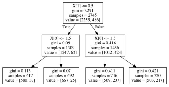
From this model, we can see that the first partition is defined by alcohol use values being <= 0.5, the subsequent partitions are both defined by biological gender <= 1.5. Starting with the entire dataset, if there is no alcohol use (variable has a value of 0) then we move to the left side of the initial partition, and we can see that there are 1309 samples for which alcohol use is recorded as none.

From this subgroup, another partition is made on biological gender, such that out of the group who are non-drinkers and who are male (617 samples), 580 of them are regular smokers, while 37 are not. In the group of non-drinkers who are female (692 samples), 667 are smokers, while 25 are not.

In the subgroup with alcohol use (1436 samples), we can see that another partition is made on biological gender. In the group of those who are male and consume alcohol (716 samples), 509 are smokers and 207 are not. In the group of those who are female and consume alcohol (720 samples), 503 are smokers and 217 are not.