srigadde

[srigadde]

Multiple Regression model

In [244]:

#import libraries import statsmodels.api import statsmodels.formula.api as smf import seaborn import matplotlib.pyplot as plt

In [245]:

#S3BQ1A10A EVER USED OTHER DRUGS #S4AQ1 EVER HAD 2-WEEK PERIOD WHEN FELT SAD, BLUE, DEPRESSED, OR DOWN MOST OF TIME # S3AQ3C1 USUAL QUANTITY WHEN SMOKED CIGARETTES #TABLIFEDX NICOTINE DEPENDENCE - LIFETIME #S2BQ2E NUMBER OF EPISODES OF ALCOHOL DEPENDENCE df=file[['S3AQ3C1','TABLIFEDX','S3BQ1A10A','S4AQ1','S2BQ2E']] #rename columns df=df.rename(columns={'S2BQ2E':'alc_dip','S3AQ3C1':'cigarettes','TABLIFEDX':'nicotine_dipendence','S3BQ1A10A':'drugs','S4AQ1':'depression'}) df.head(10)

Out[245]:cigarettesnicotine_dipendencedrugsdepressionalc_dip

0NaN022NaN

1NaN022NaN

2NaN022NaN

3NaN022NaN

4NaN022NaN

5NaN0221.0

6NaN021NaN

7NaN022NaN

8NaN021NaN

9NaN0221.0

In [263]:

#eliminate Nan Values and type modifications df.cigarettes= df.cigarettes.replace(r'^\s*$', np.nan, regex=True) df.nicotine_dipendence= df.nicotine_dipendence.replace(r'^\s*$', np.nan, regex=True) df.drugs= df.drugs.replace(r'^\s*$', np.nan, regex=True) df.depression= df.depression.replace(r'^\s*$', np.nan, regex=True) df.alc_dip= df.alc_dip.replace(r'^\s*$', np.nan, regex=True) df = df[df['cigarettes'].notna()] df = df[df['nicotine_dipendence'].notna()] df = df[df['drugs'].notna()] df = df[df['depression'].notna()] df = df[df['alc_dip'].notna()] df['cigarettes']=df['cigarettes'].astype(int) df['nicotine_dipendence']=df['nicotine_dipendence'].astype(int) df['drugs']=df['drugs'].astype(int) df['depression']=df['depression'].astype(int) df['alc_dip']=df['alc_dip'].astype(int) #eliminate unknown rows df.drop(df.index[(df["cigarettes"] == 99)|(df["alc_dip"] == 99)|(df["drugs"] == 9)|(df["depression"] == 9)],axis=0,inplace=True)

In [264]:

#replace 2 with 0 df["drugs"].replace({2: 0}, inplace=True) df["depression"].replace({2: 0}, inplace=True)

In [265]:

#subtract the mean from the explanatory variable mean=df['alc_dip'].mean() df['alc_dip']=df['alc_dip']-mean

In [266]:

df['alc_dip']=df['alc_dip'].head(500) df['cigarettes']=df['cigarettes'].head(500) df['nicotine_dipendence']=df['nicotine_dipendence'].head(500) df['drugs']=df['drugs'].head(500) df['depression']=df['depression'].head(500)

In [267]:

#regression reg=smf.ols('cigarettes~drugs+depression+alc_dip+nicotine_dipendence',data=df).fit() print(reg.summary())

                           OLS Regression Results                             ============================================================================== Dep. Variable:             cigarettes   R-squared:                       0.042 Model:                            OLS   Adj. R-squared:                  0.037 Method:                 Least Squares   F-statistic:                     7.319 Date:                Wed, 17 Feb 2021   Prob (F-statistic):           8.26e-05 Time:                        11:37:07   Log-Likelihood:                -1935.8 No. Observations:                 500   AIC:                             3880. Df Residuals:                     496   BIC:                             3896. Df Model:                           3                                         Covariance Type:            nonrobust                                         =======================================================================================                          coef    std err          t      P>|t|      [0.025      0.975] --------------------------------------------------------------------------------------- Intercept              10.8613      0.626     17.359      0.000       9.632      12.091 drugs                  -5.0872      6.764     -0.752      0.452     -18.378       8.203 depression              1.7919      0.550      3.260      0.001       0.712       2.872 alc_dip                 2.1833      0.586      3.724      0.000       1.031       3.335 nicotine_dipendence     5.0633      1.109      4.564      0.000       2.883       7.243 ============================================================================== Omnibus:                      295.837   Durbin-Watson:                   1.877 Prob(Omnibus):                  0.000   Jarque-Bera (JB):             3135.374 Skew:                           2.405   Prob(JB):                         0.00 Kurtosis:                      14.285   Cond. No.                     9.39e+15 ============================================================================== Notes: [1] Standard Errors assume that the covariance matrix of the errors is correctly specified. [2] The smallest eigenvalue is 7.69e-30. This might indicate that there are strong multicollinearity problems or that the design matrix is singular.

In [268]:

print( 'the model has coef=(1.82,2.48,4,29,2.08) and p-value(0,0.452,0,0) that suggests that there is not a strong evidence for drug and it could be a confounding variable. There is a strong collinearity which make me think about the capacity of the model so I continue with some other graphics')

the model has coef=(1.82,2.48,4,29,2.08) and p-value(0,0.452,0,0) that suggests that there is not a strong evidence for drug and it could be a confounding variable. There is a strong collinearity which make me think about the capacity of the model so I continue with some other graphics

In [269]:

## qqplot fig=statsmodels.graphics.gofplots.qqplot(reg.resid,line='r') print(' residuals do not follow normal distribution')

residuals do not follow normal distribution

In [270]:

#plot of residuals stdres=pd.DataFrame(reg.resid_pearson) fig2=plt.plot(stdres,'o',ls='None') l=plt.axhline(y=0,color='r')

In [271]:

#other regression diagnostic plot #figure=plt.figure(figsize(12,8)) #fig=statsmodels.graphics.regressionplots.plot_regress_exog(reg,'alc_dip')

In [272]:

print('the model has diffulties to intepret the response variable for the absence of normal distribution in errors.A deeper analysis is required to investigate the nature of the problem:one could be that the variable alc_dip assumes valuens between 1-98 but just values between 1 and 2 are realistic')

the model has diffulties to intepret the response variable for the absence of normal distribution in errors.A deeper analysis is required to investigate the nature of the problem:one could be that the variable alc_dip assumes valuens between 1-98 but just values between 1 and 2 are realistic

[srigadde]

Linear Regression model

Program:

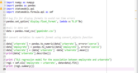
Output:

 The results of the linear regression model indicated that urbanrate (Beta= -0.1468, p= 0.000  ) was significantly and negatively associated with employrate

[srigadde]

Regression modelling - Measures

A count of the number of bicycles on each of the bridges is provided on a day-by-day basis, along with information on maximum and minimum temperature and precipitation.It assess how many bicycles cross into and out of Manhattan per day and how strongly do weather conditions affect bike volumes and the top bridge in terms of bike load.

[srigadde]

Regression modelling Data Procedure

Daily total of bike counts conducted monthly on the Brooklyn Bridge, Manhattan Bridge, Williamsburg Bridge, and Queensboro Bridge. To keep count of cyclists entering and leaving Queens, Manhattan and Brooklyn via the East River Bridges The Traffic Information Management System (TIMS) collects the count data. Each record represents the total number of cyclists per 24 hours at Brooklyn Bridge, Manhattan Bridge, Williamsburg Bridge, and Queensboro Bridge. 

[srigadde]

Regression modelling sample data

This sample data is used to measure bike utilization as a part of transportation planning. The New York City Department of Transportation collects daily data about the number of bicycles going over bridges in New York City. This dataset is a daily record of the number of bicycles crossing into or out of Manhattan via one of the East River bridges (that is, excluding Bronx thruways and the non-bikeable Hudson River tunnels) for a stretch of 9 months.