stym2801-blog

[stym2801-blog]

t3_4

[stym2801-blog]

t3_5

[stym2801-blog]

t3_3

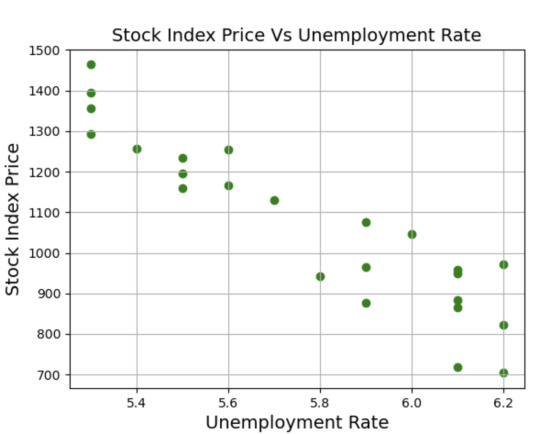
As you can see, a linear relationship also exists between the Stock_Index_Price and the Unemployment_Rate – when the unemployment rates go up, the stock index price goes down

[stym2801-blog]

t3_2

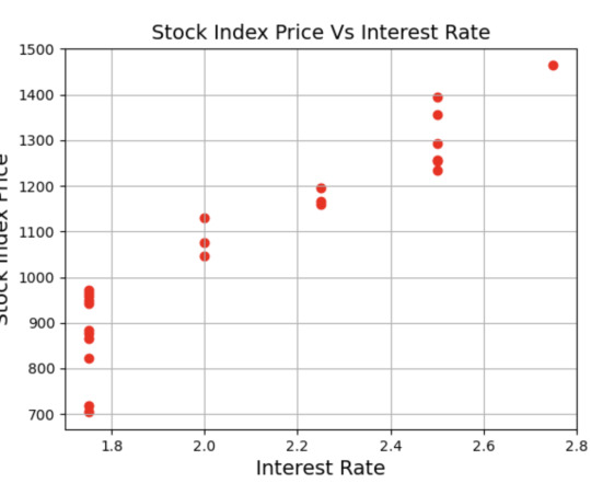
You’ll notice that indeed a linear relationship exists between the Stock_Index_Price and the Interest_Rate. Specifically, when interest rates go up, the stock index price also goes up:

[stym2801-blog]

t3_1

In the following example, we will use multiple linear regression to predict the stock index price (i.e., the dependent variable) of a fictitious economy by using 2 independent/input variables:

Interest Rate

Unemployment Rate

In our example, you may want to check that a linear relationship exists between the:

Stock_Index_Price (dependent variable) and Interest_Rate (independent variable)

Stock_Index_Price (dependent variable) and Unemployment_Rate (independent variable)

[stym2801-blog]

t1

My problem is about modeling how R&D, administration, and marketing spendings and the state will influence the profit of a company. There are 50 startups data in my dataset. 

import numpy as np

import pandas as pd

import matplotlib.pyplot as plt

dataset = pd.read_csv(“50_Startups.csv”)

X= dataset.iloc[:, :-1].values

Y=dataset.iloc[:, 4].values

from sklearn.preprocessing import LabelEncoder, OneHotEncoder

labelencoder_X = LabelEncoder()

X[: ,3]= labelencoder_X.fit_transform(X[: ,3])

onehotencoder= OneHotEncoder(categorical_features=[3])

X= onehotencoder.fit_transform(X).toarray()

X= X[:, 1:]

from sklearn.model_selection import train_test_split

X_train, X_test, Y_train, Y_test = train_test_split( X, Y, test_size=0.2, random_state=0)

from sklearn.linear_model import LinearRegression

regressor = LinearRegression()

regressor.fit(X_train,Y_train)

y_pred= regressor.predict(X_test)

[stym2801-blog]

The output of my program

[stym2801-blog]

t3

The precision is the ratio tp / (tp + fp) where tp is the number of true positives and fp the number of false positives. The precision is intuitively the ability of the classifier to not label a sample as positive if it is negative.

The recall is the ratio tp / (tp + fn) where tp is the number of true positives and fn the number of false negatives. The recall is intuitively the ability of the classifier to find all the positive samples.

The F-beta score can be interpreted as a weighted harmonic mean of the precision and recall, where an F-beta score reaches its best value at 1 and worst score at 0.

The F-beta score weights the recall more than the precision by a factor of beta. beta = 1.0 means recall and precision are equally important.

[stym2801-blog]

t2

Observations:

The average age of customers who bought the term deposit is higher than that of the customers who didn’t.

The pdays (days since the customer was last contacted) is understandably lower for the customers who bought it. The lower the pdays, the better the memory of the last call and hence the better chances of a sale.

Surprisingly, campaigns (number of contacts or calls made during the current campaign) are lower for customers who bought the term deposit.

The frequency of purchase of the deposit depends a great deal on the job title. Thus, the job title can be a good predictor of the outcome variable.

In some situations, the features have little impact on the result. So that it should be eliminated some of the independent variables to prevent the shadow on the output. We build the optimal model using Backward Elimination The backward elimination function will give us the optimal variables from my data

[stym2801-blog]

The dataset comes from the UCI Machine Learning repository, and it is related to direct marketing campaigns (phone calls) of a Portuguese banking institution. The classification goal is to predict whether the client will subscribe (1/0) to a term deposit (variable y). The dataset can be downloaded from here.

import pandas as pd

import numpy as np

from sklearn import preprocessing

import matplotlib.pyplot as plt

plt.rc("font", size=14)

from sklearn.linear_model import LogisticRegression

from sklearn.model_selection import train_test_split

import seaborn as sns

sns.set(style="white")

sns.set(style="whitegrid", color_codes=True)

The dataset provides the bank customers’ information. It includes 41,188 records and 21 fields.

Input variables

age (numeric)

job : type of job (categorical: “admin”, “blue-collar”, “entrepreneur”, “housemaid”, “management”, “retired”, “self-employed”, “services”, “student”, “technician”, “unemployed”, “unknown”)

marital : marital status (categorical: “divorced”, “married”, “single”, “unknown”)

education (categorical: “basic.4y”, “basic.6y”, “basic.9y”, “high.school”, “illiterate”, “professional.course”, “university.degree”, “unknown”)

default: has credit in default? (categorical: “no”, “yes”, “unknown”)

[stym2801-blog]

Variables

Explanatory: S1Q4A, age at first marriage.

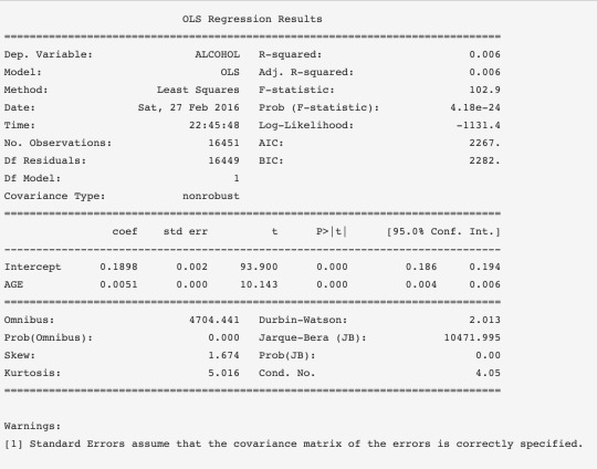
Response: ETOTLCA2, average daily volume of ethanol consumed in past year, from all types of alcoholic beverages combined.

Quantitative: 14-94 years, 31794 samples

Unknown values (99) and never married people are discarded.

Quantitative: 0.0003-219.955 oz. ethanol/day

Unkwnown values are discarded observations. Could be mapped to the mean, but don't add much.

[stym2801-blog]

RESULTS

[stym2801-blog]

Code of progr

%matplotlib inline

import numpy as np import pandas as pd import statsmodels.formula.api as smf import seaborn as sns import matplotlib.pyplot as plt

data = pd.read_csv('../datasets/NESARC/nesarc_pds.csv', usecols=['S1Q4A','ETOTLCA2'])

df = pd.DataFrame() df['AGE'] = data['S1Q4A'].replace(' ',np.NaN).replace('99',np.NaN).astype(float) df['ALCOHOL'] = data['ETOTLCA2'].replace(' ',np.NaN).astype(float) df = df.dropna()

print('Original') print(df.describe()) df['AGE'] = df['AGE']- df['AGE'].mean() print('\n\nCentered AGE') print(df.describe())

fig, (ax1,ax2)= plt.subplots(1,2) bp_age = sns.boxplot(x='AGE',data=df, whis=1.5, orient='v', ax=ax1) bp_alcohol = sns.boxplot(x='ALCOHOL',data=df, whis=1.5, orient='v', ax=(ax2)) plt.subplots_adjust(bottom=0.1, right=1.8, top=1.5) fig.show()

def outlier_limits(data, whis=1.5):    q3 = np.percentile(data, 75)    q1 = np.percentile(data, 25)    iqr = q3-q1    return(        q1-(whis*iqr),        q3+(whis*iqr),    )

[stym2801-blog]

Variables

Explanatory: S1Q4A, age at first marriage.

Response: ETOTLCA2, average daily volume of ethanol consumed in past year, from all types of alcoholic beverages combined.

Quantitative: 14-94 years, 31794 samples

Unknown values (99) and never married people are discarded.

Quantitative: 0.0003-219.955 oz. ethanol/day

Unkwnown values are discarded observations. Could be mapped to the mean, but don't add much.

[stym2801-blog]

Statistics work t3

The response variables in my investigation are the years during which I measured the unemployment rates in different countries and the  explanatory variables are the indexes of unemployment.

I found a strong connection between the level of country development and the rate of unemployment. The connection was found by creating a scatterplot  and seeing the trends between paired data.

[stym2801-blog]

Statistics work t2

I was really interested is there any connection between the level of country developing and the unemployment rate and there is. I just surfed the necessary information on this theme in the Internet and found such an useful information. The data takes 20  years starting from 2001 till 2020. The statistic information is collected in  50 countries with different level of development.

[stym2801-blog]

Statistics work t1

In my work I decided to take indexes of unemployment in twenty years in 50 European countries.

I used official statistics website for taking all the information among the years and countries.