
theresawelchy
Theresa Welchy
Theresa Welchy a Computer Systems Analyst. Theresa studies an organization's current computer systems and procedures and design information systems solutions to help the organization operate more efficiently and effectively. She brings business and information technology (IT) together by understanding the needs and limitations of both.
Check out our website
Theresa Welchy Wordpress
693 posts
Don't wanna be here? Send us removal request.
Last Seen Blogs

krystlind
even then

shatteredheartt-blog1
My heart is too broken to love again.

creeettttt
Awekmantul

the-princess-and-the-hero
She's my Princess (He's my Hero)

ayevictorino2
༶⋆˙✩ʟɪᴢᴢʏ✧‧₊˚
Text
Square Data Science Interview Questions
Square gross payment volume was 84.65 Billion U.S. dollars in 2018.

Vimarsh Karbhari
Apr 24
Square is a mobile payment company focused on credit card processing and merchant solutions. The company was founded in 2009 by Jack Dorsey — who is also Twitter’s co-founder and CEO — and Jim McKelvey, and aims to make commerce easy. Over the years, square has developed both software and hardware products, as well as business solutions to enable commerce. Square’s annual net revenue reached the 3.3 billion U.S. dollars mark in 2018, up from over 200 million U.S. dollars in 2012. Square internally has hardware, software, cash app, caviar, capital, risk and security as different teams working on technology. Data Science weaves through all these teams in different capacity. Square does billions of transactions every month and hence, each team has a huge amount of data which they can employ to generate interesting insights. Data Scientists from different domains and within fintech can find interesting work at Square.


Photo by Fancycrave on Unsplash
Interview Process
The interview process for engineering and data science follows pair programming. This answer on quora provides a good view into the Data Science teams at Square. The first step is a coding screen or a probability session. It contains writing some basic Python code in a screen sharing environment with someone from the team or answering probability based questions. That is followed by on-site interviews. The first two on-site interviews are pair programming. First one might be coding and second one on data exploration. They are followed by whiteboard interviews which consists of ML, analytics, statistics and team fit.
Important Reading
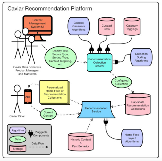

Source: Caviar Food Recommendation
Caviar Recommendation Algorithm: Recommendation Platform
Square Support Center Articles: Inferring Label Hierarchies with hLDA
Speed vs. customizability: Comparing Two Forward Feature Selection Algorithms
Data Science Related Interview Questions
How do you test whether a new credit risk scoring model works? What data would you look at?
Based on an graph drawn during the interview, what do you expect the plot of average revenue per user would look like?
Give a list of strings, find the mapping from 1–26 for each string that maximize the value for each string. Do not distinguish between capital letter and lower case, other characters do not count.
Explain your favourite ML Algorithm in detail
Consider a time series chart with a lot of ups and downs. How would you identify the peaks?
What are the different places where K-Means can be applied within Square?
Given an existing set of purchases, how do you predict the next item to purchase of a specific item?
How do you make sure you are not overfitting while training a model?
How does K-Means Algorithm work?
Explain Standard Deviation and its applications.
Reflecting on the Questions
The data science team at Square publishes articles regularly on the Squareup blog. This is an example of a modern day fintech company which does billions of transactions. The questions are geared towards how important algorithms and concepts can be applied within Square. A good creative eye for Data Science application can surely land you a job with the world’s largest retail financial transactional platform!
Subscribe to our Acing AI newsletter, I promise not to spam and its FREE!
Acing AI Newsletter — Revue
Acing AI Newsletter — Reducing the entropy in Data Science and AI. Aimed to help people get into AI and Data Science by…www.getrevue.co
Thanks for reading! 😊 If you enjoyed it, test how many times can you hit 👏 in 5 seconds. It’s great cardio for your fingers AND will help other people see the story.
The sole motivation of this blog article is to learn about Square and its technologies helping people to get into it. All data is sourced from online public sources. I aim to make this a living document, so any updates and suggested changes can always be included. Please provide relevant feedback.
DataTau published first on DataTau
0 notes
Text
How to Build an Effective Remote Team

Howdy fellas!
Never before has there been such a large number of remote employees scattered around the world. And several businesses that prefer a remote team building format still increases. It is a flexible and viable model if it is properly organized.
A work team is like a ship’s crew: everyone has a role to play in a huge effective system. A remote team is a virtual ship crew, a ship that floats in the future of work.
Like most IT companies, Standuply crew has a cozy office too, where we go to work every day. As an office team, we managed to reach considerable heights in product building, but it was time to expand the team. So we decided to set the course in the direction of remote team building and began to look for employees in other places.
Now, many months later, we know a lot about remote work: how to work from home, how to manage a remote team and how to create a business with employees who rarely see each other in real life.
Don’t get us wrong, we don’t want to say that everyone has to quit office work and start working remotely right now. We really love our office, but also we have an experience of remote team building and now want to share it with you hoping that it will help those who have not passed that hard way yet. So are you standing in front of the challenge of building a remote team and do not know where to start? Then this article is for you.
Cast off! We are going on our journey across the workflow! Remote workflow, to be specific.
Less is More

This is the first rule that you need to consider in team building with remote employees. First of all, you need to identify the people you need and what they will do. No need to recruit a lot of people, just take three persons who will be able to do the work for the five. This does not mean that three people have to work for the whole company, it means that working remotely employee performs a greater amount of work than working in the office, making the same efforts and not being distracted.
Most modern IT offices are coolly equipped, there are a lot of bean bag chairs instead of hard ones, and even hammocks, you can play kicker with colleagues, and some offices like Google’s one reminds children’s town. We do not argue with the fact that a cozy office is indeed awesome because everybody should work in comfort.
Those who go into remote work just clearly understand that work is the work, not just a kicker.
They create a comfortable area around themselves for work and they have no temptation to have snacks with employees and games. They plan when they work and rest during the remaining time.
This rule is about minimalism. Remote employees just don’t need such stuff that office gives, such as table football, and bean bag chair could be at home.
Find an ideal employee

Fifteen men on a dead man’s chest! um… startup.
Search for perfect employees, who will succeed in the project implementation and will strive to realize the global idea. Companies that hire remote employees are much more likely to find a candidate with the unique abilities necessary to perform tasks because the geographical search from one sea expands to the world ocean. There are dozens of such skills, but we have identified four main criteria, which we look at when choosing an employee:
– Yo-ho-ho and a bottle of.. enthusiasm!
Any captain wants each of the crew to share the interests of the whole ship, see him/her being proud of work and striving for common success. Enthusiasm is the fuel in the workflow ship that keeps it afloat. It all starts with an idea and desire to bring it to life. It is critical that applicants are interested in your company’s area. If a candidate at the interview did not even bother to read about the project on its official website, he/she would waste your time.
– Perfectionism (but not too much)
For a remote employee, it’s important to think critically and evaluate the work done objectively, especially if the time zone is different. Being picky and look at work as a head. The person needs to clearly understand the main goal, be able to break it into small ones and move step by step to achieve the main goal.
– Make work, not shirk
Office employees are used to working and getting paid for the time, for example from 9 to 6. Remote workers are paid not for the time, but for a result that should not be affected by any distracting things, whether it’s a sudden general cleaning or a kid who wants to watch SpongeBob right now. Or possibly it is you who want it, whatever. All this can cause the work to be completed in the last minutes before the deadline.
– Desire to work
And to learn. If the person is too lazy, has no desire to develop, and is looking for work only for money, most likely he/she is not interested in the company’s goals at all. The imaginary presence of a few working hours at the computer will not help this new fish to join the team. But what is more important is to contribute to the development of the company. It’s not gold that should keep a sailor on board.
As a rule, lazy employees are eliminated at the test task stage. If they are not really interested, they will not spend their time. You don’t need people like that.
We’ll talk more about how to cultivate these traits to go to a remote job as a job seeker and without any discomfort, but this article is not just about that.
I will call you yesterday…
Or timezones problem. Well, let’s say you found the perfect sailors on your virtual ship, but here’s the problem – time zones. If the time difference is up to 8 hours, it is almost invisible. Anyway, most of the day you are in touch with the employee.
In some cases, you will have to initially look for an employee to work at your night time, which means a time difference of 10-12 hours because the position involves working in shifts, but 24/7.
This time gap reduces the ability to call/chat during the day, so you need to allocate a couple of hours to call and give as much detail on the daily tasks for the employee to prevent possible questions to you.
What about tools?
For the most automated operation and correct processes resolution during remote team building, you will need some tools. Fortunately now on the market, you can find a lot of cool programs-assistants both paid and free and even choose by the price/functionality ratio.
– Messengers
Among messengers, we prefer Slack, of course. Our Standuply bot daily helps hundreds of teams to organize processes in Slack and to establish communication channels. Here you can read more about how to run standup meetings in Slack via Standuply. For us, this messenger is like an office: logging in Slack means coming to work.
Build a better team culture in Slack with Standuply too!

Still, of course, we use Telegram and Skype. The first is more convenient for chatting, the second one is useful for calls.
– Tasks trackers
Notebooks in the past! Use task trackers to not keep all your plans, ideas and tasks in mind. In our opinion, Asana, Trello or Jira are the most convenient ways to plan your workflow as in a diary. All tasks can be painted on the urgent or not, and forget something very difficult because everything is before my eyes. Actually, the most difficult thing is to teach each team member to use task trackers and systematically mark each step.
– Time Helper
It’s not so easy to find common work time and schedule calls with employees scattered around the world. If team members are in different time zones, you’ll need the World Clock program for Mac. In other cases, Every Time Zone or World Time Buddy will help you with time planning.
– Cloud Storage
So, in a big team, you can not deal without a storage solution which extends to cover network drives. And in that case, for us, Google Drive has no equal. It will not only free up space on your hard drive but also make it easier to communicate with your team. It is much more convenient to share a link to a document and give access to editing instead sending the same file to each other for the sake of one little edit. In addition, if your computer suddenly breaks down, you can be sure that your documents are safe in the network.
– Remote Screen Control
“Ahh! I clicked something and it’s all gone! Devs please do something!” Huh, familiar words from employees who are far from coding, aren’t they? In such a situation, it is easier to do yourself than to explain what button to press. For remote support and screen sharing, you can use a wonderful TeamViewer that allows you to control someone else’s computer and solve the problem with your own hands. Also, this program is used for remote technical support of users.
Motivation

It is hardly possible to single out a special motivation for remote employees, as for a separate type of employees. Each person’s motivation is individual, regardless of whether it is a remote or office employee. And it is important to focus on the person, analyze and to think, what is important for each one. The difference is that it’s much more difficult to understand the values and aspirations of the employee, whom you don’t see daily in the office.
Normally, it’s a set of needs, for example, an interesting area, a convenient schedule, and a decent salary. If the person is attracted only by the format of remote work or a good salary, but absolutely do not care about work itself, then it is unlikely to achieve good results.
Your sincere interest and praise even for the simplest tasks are very important for the employee’s good motivation. Did a newbie just solved a simple problem or came up with a new idea? Tell that person is doing great and you never would have come up with that yourself. Without any sarcasm, just let the employee know that he/she is important and much in the project depends. And then the person will do very best not to let you down.
Control your control

Obviously, when you build a remote team, it is difficult not to worry about the employees’ productivity. How do you know if a person is really working if you are not sitting in the same room? But actually, the problem is not about hundreds of miles between you and the employee. The problem is about lack of trust.
Some companies force remote employees to install special programs on a personal computer for time control. These are accounting systems for website traffic and counting employees’ work time. We strongly don’t support such method (and we didn’t even mention these apps in the tools section) and that’s why:
Firstly, such a distrustful attitude kills any motivation and initiative. Your employee will do the job half-heartedly and just to work off the required hours.
Secondly… Really, if there is a need to control your worker so much, do you need such worker at all? People choose remote work for freedom and the opportunity to work for the result, not for the number of hours spent on the site. Remember that your remote employees are your secret weapon.
Give your employees the freedom they are looking for and you will be surprised how effective people can work if they are not pressured.
Instead of conclusion
If you follow these uneasy rules (who said that remote team building is an easy thing?), you can assemble a remote dream team. Because the opportunities for this become more and more widespread every day. New developments are emerging, the interest of remote employees is growing, and the owners of companies are finding more and more benefits of such a solution. Remember, it is not enough to find and organize really valuable employees. They need to be interested and motivated for the best result — and this rule is applicable for any type of teams.
So good luck and may the wind be in your jib!
DataTau published first on DataTau
0 notes
Text
The Event-Driven Data Layer
Recently, I wrote an appeal to Adobe suggesting they implement first-party support for an event-driven data layer in Adobe Launch. I specifically mentioned an “event-driven, asynchronous data layer”. Let’s just call it the Event-Driven Data Layer (EDDL) to keep it simple. Since the article’s release, I’ve had a number of good conversations on this topic. The consensus seems to be that this is the right direction. For the purposes of keeping the article a manageable length, I didn’t go into too much detail of what an EDDL might look like. The goal of this article is to define what it is and why it’s a good thing.
Before we begin, let’s be clear about one thing. There’s an EDDL and a CEDDL.
CEDDL = Customer Experience Digital Data Layer. Legacy W3C.
EDDL = Event-Driven Data Layer. What this article is about.
I tried to find a less confusing abbreviation. Unfortunately, this one made the most sense. They’re both types of data layers. A good way to remember the difference is the CEDDL is 25% more cumbersome to spell and to implement. That’s being generous. The Event-Driven Data Layer describes what you’re implementing: a data layer that is constructed and transmitted to your TMS by events.
Let’s first walk through a concept that seems obvious but very few people care to think about. That is this: in a TMS, every tag is triggered by a some event. That means your pageview is triggered on an event. That event might be TMS Library Loaded (Page Top), DOM Ready, Window Loaded, or any other indication that the page has loaded. These are all events that happen on a page or screen. They are as much of an event as a click, mouseover, form submission, or anything else.
A pageview is a tag (think Adobe Analytics beacon). Viewing a page is an event. A custom link is a tag. Clicking a button is an event. Logging in is an event. Submitting a form is an event. That event might also be associated with some tags. Make sense? This is important because we need to abstract the tool from the data. Yes, you might choose to load Adobe Analytics pageview code when the window loads… but you COULD also choose to load a pageview on a click. The EDDL thinks independent of tool-specific definitions. Let’s dive into why this is the preferred method.
It’s harder to screw up
That doesn’t mean you can’t screw it up. It’s just harder to. You still need some code that sits in your header. The difference with the EDDL is:
It’s less code
You drop it in once and never have to touch it again
Maybe that means you’re simply declaring a variable (var foo = [];). Maybe it means you’re dropping in a little more code (copy/paste exercise). There’s no way around it – the variable or the function has to exist before you do anything with it. After that it’s all gravy. Timing is a non-issue with an EDDL. That’s because it proactively sends a message when a thing happens. Other data layer methodologies poll objects (like the Data Element Changed event). What does that mean?
Imagine you’re waiting on popular concert tickets to go on sale. You know what day they go on sale, but not what time. You know they’ll sell out fast, so you refresh Ticketmaster every half hour to see if their status changed. If you’re checking (or polling) to see if they’re for sale at 12:00 and they go on sale at 12:01, you might be out of luck. This is what’s called a race condition. After the status of the tickets change, you’re racing to see if you can get one before they’re gone.
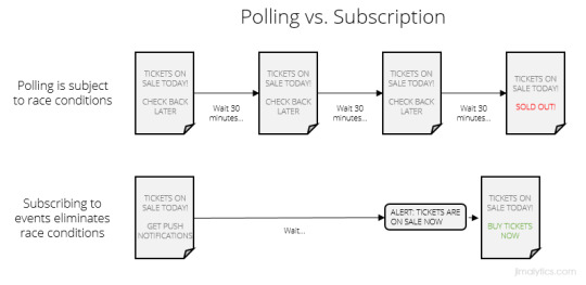
The same thing happens when you monitor data layers. If you go from Page A to Page B and you’re monitoring the object, there’s a very real chance you’ll be on the next page before your TMS realizes anything happened. That seriously sucks. You know what would fix this and save a lot of time? Subscribing to push notifications. Proactively tell me when the tickets are on sale. Don’t worry about loading the entire page object up-front. If we need to wait on servers, let me know when user information has propagated and then we’ll trigger a pageview. The EDDL uses these push notifications so you don’t have to worry about missing out on data.
It’s easier to communicate
Prioritization of data layers is difficult when it feels like a lot of work and its value isn’t immediately clear. Multiple code patterns paired with multiple sets of instructions feel like more work than one. We’re already taking focus away from the value of the data layer at this point.
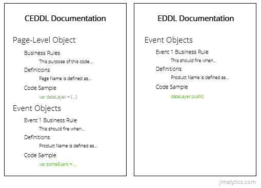
The CEDDL requires teams to learn multiple concepts/patterns. There’s a page object… and then there are events. While it might be subconscious, multiple concepts/patterns (even simple ones) requires switching mental gears. They’re also both explained as though they’re different things. Here’s an example from Adobe where both the W3C and another methodology are recommended. If I’m not very technical or I’m new to analytics, this would make my head spin.
The EDDL is much simpler. You explain it once, use the same code pattern, and can be easily dropped into a template. Here’s how the documentation might look:
Data Layer Documentation
1.0: Page and User Information
Trigger: As soon as the information is available on each page loads or screen transition.
Code: dataLayer.push({“event”:“Page Loaded”,“page”:{…}…});
1.1: Email Submit
Trigger: When a user successfully submits an email address.
Code: dataLayer.push({“event”:“Email Submit”,“attributes”:{…}…});
The documentation is consistent. We aren’t suggesting page stuff is different from event stuff. Remember that pageviews are triggered via events, too. You won’t send a pageview until you have the data you need, either. You’re not trying to figure out whether you can cram it into the header, before Page Bottom, ahead of DOM Ready, or before Window Loaded. We can just say: “When the data is there, send the pageview.” A lot of companies opted out of the W3C CEDDL for this reason alone.
It’s just as comprehensive
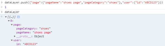
You can literally create the W3C schema with it. An effective EDDL has some kind of computed state I can access that functions like any other JSON object. What does a computed state mean, exactly? In the context of data layers, it means the content that was passed into it is processed into some kind of comprehensive object. Let’s pretend we’re using dataLayer.push() and I’m pushing information into the data layer about the page and the user. This is a Single Page App, so we will want to dynamically replace the name of the page as the user navigates. Similar to Google Tag Manager, this pushes the page and user data into the dataLayer object (because dataLayer makes more sense than digitalData):
As a business user, it’s a bit of a stretch to learn how arrays work. I just want to see what the data looks like when the page loads so I know what I can work with. That’s where a computed state is useful. As a technical stakeholder, I can advise the business user to paste dataLayer.computedState into their console to see what data is available:
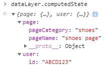
Looks like your average JSON object, right? Let’s see what happens when we want to change a field.
Side note: In hindsight, I probably should have named the pageCategory and pageName fields simply “category” and “name“. I’ll save naming convention recommendations for another post…
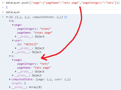
Here we’re just wanting to change the pageName and pageCategory fields. You can see the shoes data is still in that array above the hats page data. However, since that was the last information passed into the data layer, the computed state should update to reflect those changes:
There you have it. I should have the ability to add data and clear out fields, as well. For those who aren’t as technical, please note that this computed state stuff is NOT functionality baked into dataLayer.push() by default. I did some extra work to manually create the computedState object. This is for modeling purposes only. Also note that a key differentiation between this and GTM’s data layer is a publicly exposed computed state. GTM does retain a computed state, but isn’t (easily) accessible via your console.
With this functionality, the EDDL is more capable and accessible than any other client-side data layer technique.
Final Thoughts
One reason people don’t implement data layers is because it’s intimidating. You’re part of a large organization with many stakeholders. Maintaining data layer standards takes work. You’re right. Let’s also acknowledge that maintaining anything is hard and requires a certain level of discipline. There’s turnover on your team. Developers cycle in and out. Oh, by the way – you have to get this stuff prioritized, too!
The Event-Driven Data Layer is easier to document. It’s easier to implement and not as vulnerable to timing issues. It’s what a minority of sophisticated companies have already built for themselves (100 different ways) and what the majority needs to adopt. This data layer supports any schema you want. If you like how the W3C is structured, build it. If not, don’t.
One critical piece you’ll notice I didn’t link you to some EDDL library. All of this information reflects how an EDDL should behave. There are many EDDLs out there and there won’t likely be one single standard. However, Event-Driven Data Layers will eventually replace the CEDDL model. It makes more sense. I will commit to settling on a single recommendation in the coming months. There are a few examples out there:
Google Tag Manager
Data Layer Manager
If you have a public-facing event-driven data layer framework, add a comment or message me on Twitter and I would be happy to add it to this list. In the meantime, if you’re working on a data layer – don’t let the lack of a “standard” stop you from building one. If you want to use the CEDDL, go for it! Having a data layer is better than not having one.
DataTau published first on DataTau
0 notes
Text
Architectural Innovations in Convolutional Neural Networks for Image Classification
A Gentle Introduction to the Innovations in LeNet, AlexNet, VGG, Inception, and ResNet Convolutional Neural Networks.
Convolutional neural networks are comprised of two very simple elements, namely convolutional layers and pooling layers.
Although simple, there are near-infinite ways to arrange these layers for a given computer vision problem.
Fortunately, there are both common patterns for configuring these layers and architectural innovations that you can use in order to develop very deep convolutional neural networks. Studying these architectural design decisions developed for state-of-the-art image classification tasks can provide both a rationale and intuition for how to use these designs when designing your own deep convolutional neural network models.
In this tutorial, you will discover the key architecture milestones for the use of convolutional neural networks for challenging image classification problems.
After completing this tutorial, you will know:
How to pattern the number of filters and filter sizes when implementing convolutional neural networks.
How to arrange convolutional and pooling layers in a uniform pattern to develop well-performing models.
How to use the inception module and residual module to develop much deeper convolutional networks.
Let’s get started.
Tutorial Overview
This tutorial is divided into six parts; they are:
Architectural Design for CNNs
LeNet-5
AlexNet
VGG
Inception and GoogLeNet
Residual Network or ResNet
Architectural Design for CNNs
The elements of a convolutional neural network, such as convolutional and pooling layers, are relatively straightforward to understand.
The challenging part of using convolutional neural networks in practice is how to design model architectures that best use these simple elements.
A useful approach to learning how to design effective convolutional neural network architectures is to study successful applications. This is particularly straightforward to do because of the intense study and application of CNNs through 2012 to 2016 for the ImageNet Large Scale Visual Recognition Challenge, or ILSVRC. This challenge resulted in both the rapid advancement in the state of the art for very difficult computer vision tasks and the development of general innovations in the architecture of convolutional neural network models.
We will begin with the LeNet-5 that is often described as the first successful and important application of CNNs prior to the ILSVRC, then look at four different winning architectural innovations for the convolutional neural network developed for the ILSVRC, namely, AlexNet, VGG, Inception, and ResNet.
By understanding these milestone models and their architecture or architectural innovations from a high-level, you will develop both an appreciation for the use of these architectural elements in modern applications of CNN in computer vision, and be able to identify and choose architecture elements that may be useful in the design of your own models.
Want Results with Deep Learning for Computer Vision?
Take my free 7-day email crash course now (with sample code).
Click to sign-up and also get a free PDF Ebook version of the course.
Download Your FREE Mini-Course
LeNet-5
Perhaps the first widely known and successful application of convolutional neural networks was LeNet-5, described by Yann LeCun, et al. in their 1998 paper titled “Gradient-Based Learning Applied to Document Recognition” (get the PDF).
The system was developed for use in a handwritten character recognition problem and demonstrated on the MNIST standard dataset, achieving approximately 99.2% classification accuracy (or a 0.8% error rate). The network was then described as the central technique in a broader system referred to as Graph Transformer Networks.
It is a long paper, and perhaps the best part to focus on is Section II. B. that describes the LeNet-5 architecture. In the section, the paper describes the network as having seven layers with input grayscale images having the shape 32×32, the size of images in the MNIST dataset.
The model proposes a pattern of a convolutional layer followed by an average pooling layer, referred to as a subsampling layer. This pattern is repeated two and a half times before the output feature maps are flattened and fed to a number of fully connected layers for interpretation and a final prediction. A picture of the network architecture is provided in the paper and reproduced below.
Architecture of the LeNet-5 Convolutional Neural Network for Handwritten Character Recognition (taken from the 1998 paper).
The pattern of blocks of convolutional layers and pooling layers grouped together and repeated remains a common pattern in designing and using convolutional neural networks today, more than twenty years later.
Interestingly, the architecture uses a small number of filters with a very large size as the first hidden layer, specifically six filters each with the size of 28×28 pixels. After pooling, another convolutional layer has many more filters, again with a large size but smaller than the prior convolutional layer, specifically 16 filters with a size of 10×10 pixels, again followed by pooling. In the repetition of these two blocks of convolution and pooling layers, the trend is a decrease in the size of the filters, but an increase in the number of filters.
Compared to modern applications, the size of the filters is very large, as it is common to use 3×3 or similarly sized filter, and the number of filters is also small, but the trend of increasing the number of filters with the depth of the network also remains a common pattern in modern usage of the technique.
The third convolutional layer follows the first two blocks with 16 filters with a much smaller size of 5×5, although interestingly this is not followed by a pooling layer. The flattening of the feature maps and interpretation and classification of the extracted features by fully connected layers also remains a common pattern today. In modern terminology, the final section of the architecture is often referred to as the classifier, whereas the convolutional and pooling layers earlier in the model are referred to as the feature extractor.
We can summarize the key aspects of the architecture relevant in modern models as follows:
Fixed-sized input images.
Group convolutional and pooling layers into blocks.
Repetition of convolutional-pooling blocks in the architecture.
Increase in the number of features with the depth of the network.
Distinct feature extraction and classifier parts of the architecture.
AlexNet
The work that perhaps could be credited with sparking renewed interest in neural networks and the beginning of the dominance of deep learning in many computer vision applications was the 2012 paper by Alex Krizhevsky, et al. titled “ImageNet Classification with Deep Convolutional Neural Networks.”
The paper describes a model later referred to as “AlexNet” designed to address the ImageNet Large Scale Visual Recognition Challenge or ILSVRC-2010 competition for classifying photographs of objects into one of 1,000 different categories.
The ILSVRC was a competition held from 2011 to 2016, designed to spur innovation in the field of computer vision. Before the development of AlexNet, the task was thought very difficult and far beyond the capability of modern computer vision methods. AlexNet successfully demonstrated the capability of the convolutional neural network model in the domain, and kindled a fire that resulted in many more improvements and innovations, many demonstrated on the same ILSVRC task in subsequent years. More broadly, the paper showed that it is possible to develop deep and effective end-to-end models for a challenging problem without using unsupervised pretraining techniques that were popular at the time.
Important in the design of AlexNet was a suite of methods that were new or successful, but not widely adopted at the time. Now, they have become requirements when using CNNs for image classification.
AlexNet made use of the rectified linear activation function, or ReLU, as the nonlinearly after each convolutional layer, instead of S-shaped functions such as the logistic or tanh that were common up until that point. Also, a softmax activation function was used in the output layer, now a staple for multi-class classification with neural networks.
The average pooling used in LeNet-5 was replaced with a max pooling method, although in this case, overlapping pooling was found to outperform non-overlapping pooling that is commonly used today (e.g. stride of pooling operation is the same size as the pooling operation, e.g. 2 by 2 pixels). To address overfitting, the newly proposed dropout method was used between the fully connected layers of the classifier part of the model to improve generalization error.
The architecture of AlexNet is deep and extends upon some of the patterns established with LeNet-5. The image below, taken from the paper, summarizes the model architecture, in this case, split into two pipelines to train on the GPU hardware of the time.
Architecture of the AlexNet Convolutional Neural Network for Object Photo Classification (taken from the 2012 paper).
The model has five convolutional layers in the feature extraction part of the model and three fully connected layers in the classifier part of the model.
Input images were fixed to the size 224×224 with three color channels. In terms of the number of filters used in each convolutional layer, the pattern of increasing the number of filters with depth seen in LeNet was mostly adhered to, in this case, the sizes: 96, 256, 384, 384, and 256. Similarly, the pattern of decreasing the size of the filter (kernel) with depth was used, starting from the smaller size of 11×11 and decreasing to 5×5, and then to 3×3 in the deeper layers. Use of small filters such as 5×5 and 3×3 is now the norm.
A pattern of a convolutional layer followed by pooling layer was used at the start and end of the feature detection part of the model. Interestingly, a pattern of convolutional layer followed immediately by a second convolutional layer was used. This pattern too has become a modern standard.
The model was trained with data augmentation, artificially increasing the size of the training dataset and giving the model more of an opportunity to learn the same features in different orientations.
We can summarize the key aspects of the architecture relevant in modern models as follows:
Use of the ReLU activation function after convolutional layers and softmax for the output layer.
Use of Max Pooling instead of Average Pooling.
Use of Dropout regularization between the fully connected layers.
Pattern of convolutional layer fed directly to another convolutional layer.
Use of Data Augmentation.
VGG
The development of deep convolutional neural networks for computer vision tasks appeared to be a little bit of a dark art after AlexNet.
An important work that sought to standardize architecture design for deep convolutional networks and developed much deeper and better performing models in the process was the 2014 paper titled “Very Deep Convolutional Networks for Large-Scale Image Recognition” by Karen Simonyan and Andrew Zisserman.
Their architecture is generally referred to as VGG after the name of their lab, the Visual Geometry Group at Oxford. Their model was developed and demonstrated on the sameILSVRC competition, in this case, the ILSVRC-2014 version of the challenge.
The first important difference that has become a de facto standard is the use of a large number of small filters. Specifically, filters with the size 3×3 and 1×1 with the stride of one, different from the large sized filters in LeNet-5 and the smaller but still relatively large filters and large stride of four in AlexNet.
Max pooling layers are used after most, but not all, convolutional layers, learning from the example in AlexNet, yet all pooling is performed with the size 2×2 and the same stride, that too has become a de facto standard. Specifically, the VGG networks use examples of two, three, and even four convolutional layers stacked together before a max pooling layer is used. The rationale was that stacked convolutional layers with smaller filters approximate the effect of one convolutional layer with a larger sized filter, e.g. three stacked convolutional layers with 3×3 filters approximates one convolutional layer with a 7×7 filter.
Another important difference is the very large number of filters used. The number of filters increases with the depth of the model, although starts at a relatively large number of 64 and increases through 128, 256, and 512 filters at the end of the feature extraction part of the model.
A number of variants of the architecture were developed and evaluated, although two are referred to most commonly given their performance and depth. They are named for the number of layers: they are the VGG-16 and the VGG-19 for 16 and 19 learned layers respectively.
Below is a table taken from the paper; note the two far right columns indicating the configuration (number of filters) used in the VGG-16 and VGG-19 versions of the architecture.
Architecture of the VGG Convolutional Neural Network for Object Photo Classification (taken from the 2014 paper).
The design decisions in the VGG models have become the starting point for simple and direct use of convolutional neural networks in general.
Finally, the VGG work was among the first to release the valuable model weights under a permissive license that led to a trend among deep learning computer vision researchers. This, in turn, has led to the heavy use of pre-trained models like VGG in transfer learning as a starting point on new computer vision tasks.
We can summarize the key aspects of the architecture relevant in modern models as follows:
Use of very small convolutional filters, e.g. 3×3 and 1×1 with a stride of one.
Use of max pooling with a size of 2×2 and a stride of the same dimensions.
The importance of stacking convolutional layers together before using a pooling layer to define a block.
Dramatic repetition of the convolutional-pooling block pattern.
Development of very deep (16 and 19 layer) models.
Inception and GoogLeNet
Important innovations in the use of convolutional layers were proposed in the 2015 paper by Christian Szegedy, et al. titled “Going Deeper with Convolutions.”
In the paper, the authors propose an architecture referred to as inception (or inception v1 to differentiate it from extensions) and a specific model called GoogLeNet that achieved top results in the 2014 version of the ILSVRC challenge.
The key innovation on the inception models is called the inception module. This is a block of parallel convolutional layers with different sized filters (e.g. 1×1, 3×3, 5×5) and a 3×3 max pooling layer, the results of which are then concatenated. Below is an example of the inception module taken from the paper.
Example of the Naive Inception Module (taken from the 2015 paper).
A problem with a naive implementation of the inception model is that the number of filters (depth or channels) begins to build up fast, especially when inception modules are stacked.
Performing convolutions with larger filter sizes (e.g. 3 and 5) can be computationally expensive on a large number of filters. To address this, 1×1 convolutional layers are used to reduce the number of filters in the inception model. Specifically before the 3×3 and 5×5 convolutional layers and after the pooling layer. The image below taken from the paper shows this change to the inception module.
Example of the Inception Module With Dimensionality Reduction (taken from the 2015 paper).
A second important design decision in the inception model was connecting the output at different points in the model. This was achieved by creating small off-shoot output networks from the main network that were trained to make a prediction. The intent was to provide an additional error signal from the classification task at different points of the deep model in order to address the vanishing gradients problem. These small output networks were then removed after training.
Below shows a rotated version (left-to-right for input-to-output) of the architecture of the GoogLeNet model taken from the paper using the Inception modules from the input on the left to the output classification on the right and the two additional output networks that were only used during training.
Architecture of the GoogLeNet Model Used During Training for Object Photo Classification (taken from the 2015 paper).
Interestingly, overlapping max pooling was used and a large average pooling operation was used at the end of the feature extraction part of the model prior to the classifier part of the model.
We can summarize the key aspects of the architecture relevant in modern models as follows:
Development and repetition of the Inception module.
Heavy use of the 1×1 convolution to reduce the number of channels.
Use of error feedback at multiple points in the network.
Development of very deep (22-layer) models.
Use of global average pooling for the output of the model.
Residual Network or ResNet
A final important innovation in convolutional neural nets that we will review was proposed by Kaiming He, et al. in their 2016 paper titled “Deep Residual Learning for Image Recognition.”
In the paper, the authors proposed a very deep model called a Residual Network, or ResNet for short, an example of which achieved success on the 2015 version of the ILSVRC challenge.
Their model had an impressive 152 layers. Key to the model design is the idea of residual blocks that make use of shortcut connections. These are simply connections in the network architecture where the input is kept as-is (not weighted) and passed on to a deeper layer, e.g. skipping the next layer.
A residual block is a pattern of two convolutional layers with ReLU activation where the output of the block is combined with the input to the block, e.g. the shortcut connection. A projected version of the input used via 1×1 if the shape of the input to the block is different to the output of the block, so-called 1×1 convolutions. These are referred to as projected shortcut connections, compared to the unweighted or identity shortcut connections.
The authors start with what they call a plain network, which is a VGG-inspired deep convolutional neural network with small filters (3×3), grouped convolutional layers followed with no pooling in between, and an average pooling at the end of the feature detector part of the model prior to the fully connected output layer with a softmax activation function.
The plain network is modified to become a residual network by adding shortcut connections in order to define residual blocks. Typically the shape of the input for the shortcut connection is the same size as the output of the residual block.
The image below was taken from the paper and from left to right compares the architecture of a VGG model, a plain convolutional model, and a version of the plain convolutional with residual modules, called a residual network.
Architecture of the Residual Network for Object Photo Classification (taken from the 2016 paper).
We can summarize the key aspects of the architecture relevant in modern models as follows:
Use of shortcut connections.
Development and repetition of the residual blocks.
Development of very deep (152-layer) models.
Further Reading
This section provides more resources on the topic if you are looking to go deeper.
Papers
Gradient-based learning applied to document recognition, (PDF) 1998.
ImageNet Classification with Deep Convolutional Neural Networks, 2012.
Very Deep Convolutional Networks for Large-Scale Image Recognition, 2014.
Going Deeper with Convolutions, 2015.
Deep Residual Learning for Image Recognition, 2016
API
Keras Applications API
Articles
The 9 Deep Learning Papers You Need To Know About
A Simple Guide to the Versions of the Inception Network, 2018.
CNN Architectures: LeNet, AlexNet, VGG, GoogLeNet, ResNet and more., 2017.
Summary
In this tutorial, you discovered the key architecture milestones for the use of convolutional neural networks for challenging image classification.
Specifically, you learned:
How to pattern the number of filters and filter sizes when implementing convolutional neural networks.
How to arrange convolutional and pooling layers in a uniform pattern to develop well-performing models.
How to use the inception module and residual module to develop much deeper convolutional networks.
Do you have any questions?
Ask your questions in the comments below and I will do my best to answer.
The post Architectural Innovations in Convolutional Neural Networks for Image Classification appeared first on Machine Learning Mastery.
Machine Learning Mastery published first on Machine Learning Mastery
0 notes
Text
Quiz Show Scandals/Admissions Scandal/Stormy Daniels/Beer names:being a lawyer would drive me nuts!!!!!!
0) Charles van Doren (see here) passed away recently. For those who don't know he he was (prob most of you) he was one of the contestants involved in RIGGED quiz shows in the 1950's. While there was a Grand Jury Hearing about Quiz Shows being rigged, nobody went to jail since TV was new and it was not clear if rigging quiz shows was illegal. Laws were then passed to make them it illegal.
So why are today's so-called reality shows legal? I ask non-rhetorically.
(The person he beat in a rigged game show- Herb Stempel (see here) is still alive.)
1) The college admissions scandal. I won't restate the details and how awful it is since you can get that elsewhere and I doubt I can add much to it. One thing I've heard in the discussions about it is a question that is often posted rhetorically but I want to pose for real:
There are people whose parents give X dollars to a school and they get admitted even though they are not qualified. Why is that legal?
I ask that question without an ax to grind and without anger. Why is out-right bribery of this sort legal?
Possibilities:
a) Its transparent. So being honest about bribery makes it okay?
b) My question said `even though they are not qualified' - what if they explicitly or implicitly said `having parents give money to our school is one of our qualifications'
c) The money they give is used to fund scholarships for students who can't afford to go. This is an argument for why its not immoral, not why its not illegal.
But here is my question: Really, what is the legal issue here? It still seems like bribery.
2) Big Oil gives money to congressman Smith, who then votes against a carbon tax. This seems like outright bribery
Caveat:
a) If Congressman Smith is normally a anti-regulation then he could say correctly that he was given the money because they agree with his general philosophy, so it's not bribery.
b) If Congressman smith is normally pro-environment and has no problem with voting for taxes then perhaps it is bribery.
3) John Edwards a while back and Donald Trump now are claiming (not quite) that the money used to pay off their mistress to be quiet is NOT a campaign contribution, but was to keep the affair from his wife. (I don't think Donald Trump has admitted the affair so its harder to know what his defense is). But lets take a less controversial example of `what is a campaign contribution'
I throw a party for my wife's 50th birthday and I invite Beto O'Rourke and many voters and some Dem party big-wigs to the party. The party costs me $50,000. While I claim it's for my wife's bday it really is for Beto to make connections to voters and others. So is that a campaign contribution?
4) The creators of HUGE ASS BEER are suing GIANT ASS BEER for trademark infringement. I am not making this up- see here
---------------------------------------------------------
All of these cases involve ill defined questions (e.g., `what is a bribe'). And the people arguing either side are not unbiased. The cases also illustrate why I prefer mathematics: nice clean questions that (for the most part) have answers. We may have our biases as to which way they go, but if it went the other way we would not sue in a court of law.
Computational Complexity published first on Computational Complexity
0 notes
Text
End of term
We’ve reached the end of term again on The Morning Paper, and I’ll be taking a two week break. The Morning Paper will resume on Tuesday 7th May (since Monday 6th is a public holiday in the UK).
My end of term tradition is to highlight a few of the papers from the term that I especially enjoyed, but this time around I want to let one work stand alone:
Making reliable distributed systems in the presence of software errors, Joe Armstrong, December 2003.
You might also enjoy “The Mess We’re In,” and Joe’s seven deadly sins of programming:
Code even you cannot understand a week after you wrote it – no comments
Code with no specifications
Code that is shipped as soon as it runs and before it is beautiful
Code with added features
Code that is very very fast very very very obscure and incorrect
Code that is not beautiful
Code that you wrote without understanding the problem
We’re in an even bigger mess without you Joe. Thank you for everything. RIP.
the morning paper published first on the morning paper
0 notes
Text
A Gentle Introduction to Pooling Layers for Convolutional Neural Networks
Convolutional layers in a convolutional neural network summarize the presence of features in an input image.
A problem with the output feature maps is that they are sensitive to the location of the features in the input. One approach to address this sensitivity is to down sample the feature maps. This has the effect of making the resulting down sampled feature maps more robust to changes in the position of the feature in the image, referred to by the technical phrase “local translation invariance.”
Pooling layers provide an approach to down sampling feature maps by summarizing the presence of features in patches of the feature map. Two common pooling methods are average pooling and max pooling that summarize the average presence of a feature and the most activated presence of a feature respectively.
In this tutorial, you will discover how the pooling operation works and how to implement it in convolutional neural networks.
After completing this tutorial, you will know:
Pooling is required to down sample the detection of features in feature maps.
How to calculate and implement average and maximum pooling in a convolutional neural network.
How to use global pooling in a convolutional neural network.
Let’s get started.
A Gentle Introduction to Pooling Layers for Convolutional Neural Networks
Photo by Nicholas A. Tonelli, some rights reserved.
Tutorial Overview
This tutorial is divided into five parts; they are:
Pooling
Detecting Vertical Lines
Average Pooling Layers
Max Pooling Layers
Global Pooling Layers
Want Results with Deep Learning for Computer Vision?
Take my free 7-day email crash course now (with sample code).
Click to sign-up and also get a free PDF Ebook version of the course.
Download Your FREE Mini-Course
Pooling Layers
Convolutional layers in a convolutional neural network systematically apply learned filters to input images in order to create feature maps that summarize the presence of those features in the input.
Convolutional layers prove very effective, and stacking convolutional layers in deep models allows layers close to the input to learn low-level features (e.g. lines) and layers deeper in the model to learn high-order or more abstract features, like shapes or specific objects.
A limitation of the feature map output of convolutional layers is that they record the precise position of features in the input. This means that small movements in the position of the feature in the input image will result in a different feature map. This can happen with re-cropping, rotation, shifting, and other minor changes to the input image.
A common approach to addressing this problem from signal processing is called down sampling. This is where a lower resolution version of an input signal is created that still contains the large or important structural elements, without the fine detail that may not be as useful to the task.
Down sampling can be achieved with convolutional layers by changing the stride of the convolution across the image. A more robust and common approach is to use a pooling layer.
A pooling layer is a new layer added after the convolutional layer. Specifically, after a nonlinearity (e.g. ReLU) has been applied to the feature maps output by a convolutional layer; for example the layers in a model may look as follows:
Input Image
Convolutional Layer
Nonlinearity
Pooling Layer
The addition of a pooling layer after the convolutional layer is a common pattern used for ordering layers within a convolutional neural network that may be repeated one or more times in a given model.
The pooling layer operates upon each feature map separately to create a new set of the same number of pooled feature maps.
Pooling involves selecting a pooling operation, much like a filter to be applied to feature maps. The size of the pooling operation or filter is smaller than the size of the feature map; specifically, it is almost always 2×2 pixels applied with a stride of 2 pixels.
This means that the pooling layer will always reduce the size of each feature map by a factor of 2, e.g. each dimension is halved, reducing the number of pixels or values in each feature map to one quarter the size. For example, a pooling layer applied to a feature map of 6×6 (36 pixels) will result in an output pooled feature map of 3×3 (9 pixels).
The pooling operation is specified, rather than learned. Two common functions used in the pooling operation are:
Average Pooling: Calculate the average value for each patch on the feature map.
Maximum Pooling (or Max Pooling): Calculate the maximum value for each patch of the feature map.
The result of using a pooling layer and creating down sampled or pooled feature maps is a summarized version of the features detected in the input. They are useful as small changes in the location of the feature in the input detected by the convolutional layer will result in a pooled feature map with the feature in the same location. This capability added by pooling is called the model’s invariance to local translation.
In all cases, pooling helps to make the representation become approximately invariant to small translations of the input. Invariance to translation means that if we translate the input by a small amount, the values of most of the pooled outputs do not change.
— Page 342, Deep Learning, 2016.
Now that we are familiar with the need and benefit of pooling layers, let’s look at some specific examples.
Detecting Vertical Lines
Before we look at some examples of pooling layers and their effects, let’s develop a small example of an input image and convolutional layer to which we can later add and evaluate pooling layers.
In this example, we define a single input image or sample that has one channel and is an 8 pixel by 8 pixel square with all 0 values and a two-pixel wide vertical line in the center.
# define input data data = [[0, 0, 0, 1, 1, 0, 0, 0], [0, 0, 0, 1, 1, 0, 0, 0], [0, 0, 0, 1, 1, 0, 0, 0], [0, 0, 0, 1, 1, 0, 0, 0], [0, 0, 0, 1, 1, 0, 0, 0], [0, 0, 0, 1, 1, 0, 0, 0], [0, 0, 0, 1, 1, 0, 0, 0], [0, 0, 0, 1, 1, 0, 0, 0]] data = asarray(data) data = data.reshape(1, 8, 8, 1)
Next, we can define a model that expects input samples to have the shape (8, 8, 1) and has a single hidden convolutional layer with a single filter with the shape of 3 pixels by 3 pixels.
A rectified linear activation function, or ReLU for short, is then applied to each value in the feature map. This is a simple and effective nonlinearity, that in this case will not change the values in the feature map, but is present because we will later add subsequent pooling layers and pooling is added after the nonlinearity applied to the feature maps, e.g. a best practice.
# create model model = Sequential() model.add(Conv2D(1, (3,3), activation='relu', input_shape=(8, 8, 1))) # summarize model model.summary()
The filter is initialized with random weights as part of the initialization of the model.
Instead, we will hard code our own 3×3 filter that will detect vertical lines. That is the filter will strongly activate when it detects a vertical line and weakly activate when it does not. We expect that by applying this filter across the input image that the output feature map will show that the vertical line was detected.
# define a vertical line detector detector = [[[[0]],[[1]],[[0]]], [[[0]],[[1]],[[0]]], [[[0]],[[1]],[[0]]]] weights = [asarray(detector), asarray([0.0])] # store the weights in the model model.set_weights(weights)
Next, we can apply the filter to our input image by calling the predict() function on the model.
# apply filter to input data yhat = model.predict(data)
The result is a four-dimensional output with one batch, a given number of rows and columns, and one filter, or [batch, rows, columns, filters]. We can print the activations in the single feature map to confirm that the line was detected.
# enumerate rows for r in range(yhat.shape[1]): # print each column in the row print([yhat[0,r,c,0] for c in range(yhat.shape[2])])
Tying all of this together, the complete example is listed below.
# example of vertical line detection with a convolutional layer from numpy import asarray from keras.models import Sequential from keras.layers import Conv2D # define input data data = [[0, 0, 0, 1, 1, 0, 0, 0], [0, 0, 0, 1, 1, 0, 0, 0], [0, 0, 0, 1, 1, 0, 0, 0], [0, 0, 0, 1, 1, 0, 0, 0], [0, 0, 0, 1, 1, 0, 0, 0], [0, 0, 0, 1, 1, 0, 0, 0], [0, 0, 0, 1, 1, 0, 0, 0], [0, 0, 0, 1, 1, 0, 0, 0]] data = asarray(data) data = data.reshape(1, 8, 8, 1) # create model model = Sequential() model.add(Conv2D(1, (3,3), activation='relu', input_shape=(8, 8, 1))) # summarize model model.summary() # define a vertical line detector detector = [[[[0]],[[1]],[[0]]], [[[0]],[[1]],[[0]]], [[[0]],[[1]],[[0]]]] weights = [asarray(detector), asarray([0.0])] # store the weights in the model model.set_weights(weights) # apply filter to input data yhat = model.predict(data) # enumerate rows for r in range(yhat.shape[1]): # print each column in the row print([yhat[0,r,c,0] for c in range(yhat.shape[2])])
Running the example first summarizes the structure of the model.
Of note is that the single hidden convolutional layer will take the 8×8 pixel input image and will produce a feature map with the dimensions of 6×6.
We can also see that the layer has 10 parameters: that is nine weights for the filter (3×3) and one weight for the bias.
Finally, the single feature map is printed.
We can see from reviewing the numbers in the 6×6 matrix that indeed the manually specified filter detected the vertical line in the middle of our input image.
_________________________________________________________________ Layer (type) Output Shape Param # ================================================================= conv2d_1 (Conv2D) (None, 6, 6, 1) 10 ================================================================= Total params: 10 Trainable params: 10 Non-trainable params: 0 _________________________________________________________________ [0.0, 0.0, 3.0, 3.0, 0.0, 0.0] [0.0, 0.0, 3.0, 3.0, 0.0, 0.0] [0.0, 0.0, 3.0, 3.0, 0.0, 0.0] [0.0, 0.0, 3.0, 3.0, 0.0, 0.0] [0.0, 0.0, 3.0, 3.0, 0.0, 0.0] [0.0, 0.0, 3.0, 3.0, 0.0, 0.0]
We can now look at some common approaches to pooling and how they impact the output feature maps.
Average Pooling Layer
On two-dimensional feature maps, pooling is typically applied in 2×2 patches of the feature map with a stride of (2,2).
Average pooling involves calculating the average for each patch of the feature map. This means that each 2×2 square of the feature map is down sampled to the average value in the square.
For example, the output of the line detector convolutional filter in the previous section was a 6×6 feature map. We can look at applying the average pooling operation to the first line of that feature map manually.
The first line for pooling (first two rows and six columns) of the output feature map were as follows:
[0.0, 0.0, 3.0, 3.0, 0.0, 0.0] [0.0, 0.0, 3.0, 3.0, 0.0, 0.0]
The first pooling operation is applied as follows:
average(0.0, 0.0) = 0.0 0.0, 0.0
Given the stride of two, the operation is moved along two columns to the left and the average is calculated:
average(3.0, 3.0) = 3.0 3.0, 3.0
Again, the operation is moved along two columns to the left and the average is calculated:
average(0.0, 0.0) = 0.0 0.0, 0.0
That’s it for the first line of pooling operations. The result is the first line of the average pooling operation:
[0.0, 3.0, 0.0]
Given the (2,2) stride, the operation would then be moved down two rows and back to the first column and the process continued.
Because the downsampling operation halves each dimension, we will expect the output of pooling applied to the 6×6 feature map to be a new 3×3 feature map. Given the horizontal symmetry of the feature map input, we would expect each row to have the same average pooling values. Therefore, we would expect the resulting average pooling of the detected line feature map from the previous section to look as follows:
[0.0, 3.0, 0.0] [0.0, 3.0, 0.0] [0.0, 3.0, 0.0]
We can confirm this by updating the example from the previous section to use average pooling.
This can be achieved in Keras by using the AveragePooling2D layer. The default pool_size (e.g. like the kernel size or filter size) of the layer is (2,2) and the default strides is None, which in this case means using the pool_size as the strides, which will be (2,2).
# create model model = Sequential() model.add(Conv2D(1, (3,3), activation='relu', input_shape=(8, 8, 1))) model.add(AveragePooling2D())
The complete example with average pooling is listed below.
# example of average pooling from numpy import asarray from keras.models import Sequential from keras.layers import Conv2D from keras.layers import AveragePooling2D # define input data data = [[0, 0, 0, 1, 1, 0, 0, 0], [0, 0, 0, 1, 1, 0, 0, 0], [0, 0, 0, 1, 1, 0, 0, 0], [0, 0, 0, 1, 1, 0, 0, 0], [0, 0, 0, 1, 1, 0, 0, 0], [0, 0, 0, 1, 1, 0, 0, 0], [0, 0, 0, 1, 1, 0, 0, 0], [0, 0, 0, 1, 1, 0, 0, 0]] data = asarray(data) data = data.reshape(1, 8, 8, 1) # create model model = Sequential() model.add(Conv2D(1, (3,3), activation='relu', input_shape=(8, 8, 1))) model.add(AveragePooling2D()) # summarize model model.summary() # define a vertical line detector detector = [[[[0]],[[1]],[[0]]], [[[0]],[[1]],[[0]]], [[[0]],[[1]],[[0]]]] weights = [asarray(detector), asarray([0.0])] # store the weights in the model model.set_weights(weights) # apply filter to input data yhat = model.predict(data) # enumerate rows for r in range(yhat.shape[1]): # print each column in the row print([yhat[0,r,c,0] for c in range(yhat.shape[2])])
Running the example first summarizes the model.
We can see from the model summary that the input to the pooling layer will be a single feature map with the shape (6,6) and that the output of the average pooling layer will be a single feature map with each dimension halved, with the shape (3,3).
Applying the average pooling results in a new feature map that still detects the line, although in a down sampled manner, exactly as we expected from calculating the operation manually.
_________________________________________________________________ Layer (type) Output Shape Param # ================================================================= conv2d_1 (Conv2D) (None, 6, 6, 1) 10 _________________________________________________________________ average_pooling2d_1 (Average (None, 3, 3, 1) 0 ================================================================= Total params: 10 Trainable params: 10 Non-trainable params: 0 _________________________________________________________________ [0.0, 3.0, 0.0] [0.0, 3.0, 0.0] [0.0, 3.0, 0.0]
Average pooling works well, although it is more common to use max pooling.
Max Pooling Layer
Maximum pooling, or max pooling, is a pooling operation that calculates the maximum, or largest, value in each patch of each feature map.
The results are down sampled or pooled feature maps that highlight the most present feature in the patch, not the average presence of the feature in the case of average pooling. This has been found to work better in practice than average pooling for computer vision tasks like image classification.
In a nutshell, the reason is that features tend to encode the spatial presence of some pattern or concept over the different tiles of the feature map (hence, the term feature map), and it’s more informative to look at the maximal presence of different features than at their average presence.
— Page 129, Deep Learning with Python, 2017.
We can make the max pooling operation concrete by again applying it to the output feature map of the line detector convolutional operation and manually calculate the first row of the pooled feature map.
The first line for pooling (first two rows and six columns) of the output feature map were as follows:
[0.0, 0.0, 3.0, 3.0, 0.0, 0.0] [0.0, 0.0, 3.0, 3.0, 0.0, 0.0]
The first max pooling operation is applied as follows:
max(0.0, 0.0) = 0.0 0.0, 0.0
Given the stride of two, the operation is moved along two columns to the left and the max is calculated:
max(3.0, 3.0) = 3.0 3.0, 3.0
Again, the operation is moved along two columns to the left and the max is calculated:
max(0.0, 0.0) = 0.0 0.0, 0.0
That’s it for the first line of pooling operations.
The result is the first line of the max pooling operation:
[0.0, 3.0, 0.0]
Again, given the horizontal symmetry of the feature map provided for pooling, we would expect the pooled feature map to look as follows:
[0.0, 3.0, 0.0] [0.0, 3.0, 0.0] [0.0, 3.0, 0.0]
It just so happens that the chosen line detector image and feature map produce the same output when downsampled with average pooling and maximum pooling.
The maximum pooling operation can be added to the worked example by adding the MaxPooling2D layer provided by the Keras API.
# create model model = Sequential() model.add(Conv2D(1, (3,3), activation='relu', input_shape=(8, 8, 1))) model.add(MaxPooling2D())
The complete example of vertical line detection with max pooling is listed below.
# example of max pooling from numpy import asarray from keras.models import Sequential from keras.layers import Conv2D from keras.layers import MaxPooling2D # define input data data = [[0, 0, 0, 1, 1, 0, 0, 0], [0, 0, 0, 1, 1, 0, 0, 0], [0, 0, 0, 1, 1, 0, 0, 0], [0, 0, 0, 1, 1, 0, 0, 0], [0, 0, 0, 1, 1, 0, 0, 0], [0, 0, 0, 1, 1, 0, 0, 0], [0, 0, 0, 1, 1, 0, 0, 0], [0, 0, 0, 1, 1, 0, 0, 0]] data = asarray(data) data = data.reshape(1, 8, 8, 1) # create model model = Sequential() model.add(Conv2D(1, (3,3), activation='relu', input_shape=(8, 8, 1))) model.add(MaxPooling2D()) # summarize model model.summary() # define a vertical line detector detector = [[[[0]],[[1]],[[0]]], [[[0]],[[1]],[[0]]], [[[0]],[[1]],[[0]]]] weights = [asarray(detector), asarray([0.0])] # store the weights in the model model.set_weights(weights) # apply filter to input data yhat = model.predict(data) # enumerate rows for r in range(yhat.shape[1]): # print each column in the row print([yhat[0,r,c,0] for c in range(yhat.shape[2])])
Running the example first summarizes the model.
We can see, as we might expect by now, that the output of the max pooling layer will be a single feature map with each dimension halved, with the shape (3,3).
Applying the max pooling results in a new feature map that still detects the line, although in a down sampled manner.
_________________________________________________________________ Layer (type) Output Shape Param # ================================================================= conv2d_1 (Conv2D) (None, 6, 6, 1) 10 _________________________________________________________________ max_pooling2d_1 (MaxPooling2 (None, 3, 3, 1) 0 ================================================================= Total params: 10 Trainable params: 10 Non-trainable params: 0 _________________________________________________________________ [0.0, 3.0, 0.0] [0.0, 3.0, 0.0] [0.0, 3.0, 0.0]
Global Pooling Layers
There is another type of pooling that is sometimes used called global pooling.
Instead of down sampling patches of the input feature map, global pooling down samples the entire feature map to a single value. This would be the same as setting the pool_size to the size of the input feature map.
Global pooling can be used in a model to aggressively summarize the presence of a feature in an image. It is also sometimes used in models as an alternative to using a fully connected layer to transition from feature maps to an output prediction for the model.
Both global average pooling and global max pooling are supported by Keras via the GlobalAveragePooling2D and GlobalMaxPooling2D classes respectively.
For example, we can add global max pooling to the convolutional model used for vertical line detection.
# create model model = Sequential() model.add(Conv2D(1, (3,3), activation='relu', input_shape=(8, 8, 1))) model.add(GlobalMaxPooling2D())
The outcome will be a single value that will summarize the strongest activation or presence of the vertical line in the input image.
The complete code listing is provided below.
# example of using global max pooling from numpy import asarray from keras.models import Sequential from keras.layers import Conv2D from keras.layers import GlobalMaxPooling2D # define input data data = [[0, 0, 0, 1, 1, 0, 0, 0], [0, 0, 0, 1, 1, 0, 0, 0], [0, 0, 0, 1, 1, 0, 0, 0], [0, 0, 0, 1, 1, 0, 0, 0], [0, 0, 0, 1, 1, 0, 0, 0], [0, 0, 0, 1, 1, 0, 0, 0], [0, 0, 0, 1, 1, 0, 0, 0], [0, 0, 0, 1, 1, 0, 0, 0]] data = asarray(data) data = data.reshape(1, 8, 8, 1) # create model model = Sequential() model.add(Conv2D(1, (3,3), activation='relu', input_shape=(8, 8, 1))) model.add(GlobalMaxPooling2D()) # summarize model model.summary() # # define a vertical line detector detector = [[[[0]],[[1]],[[0]]], [[[0]],[[1]],[[0]]], [[[0]],[[1]],[[0]]]] weights = [asarray(detector), asarray([0.0])] # store the weights in the model model.set_weights(weights) # apply filter to input data yhat = model.predict(data) # enumerate rows print(yhat)
Running the example first summarizes the model
We can see that, as expected, the output of the global pooling layer is a single value that summarizes the presence of the feature in the single feature map.
Next, the output of the model is printed showing the effect of global max pooling on the feature map, printing the single largest activation.
_________________________________________________________________ Layer (type) Output Shape Param # ================================================================= conv2d_1 (Conv2D) (None, 6, 6, 1) 10 _________________________________________________________________ global_max_pooling2d_1 (Glob (None, 1) 0 ================================================================= Total params: 10 Trainable params: 10 Non-trainable params: 0 _________________________________________________________________ [[3.]]
Further Reading
This section provides more resources on the topic if you are looking to go deeper.
Posts
Crash Course in Convolutional Neural Networks for Machine Learning
Books
Chapter 9: Convolutional Networks, Deep Learning, 2016.
Chapter 5: Deep Learning for Computer Vision, Deep Learning with Python, 2017.
API
Keras Convolutional Layers API
Keras Pooling Layers API
Summary
In this tutorial, you discovered how the pooling operation works and how to implement it in convolutional neural networks.
Specifically, you learned:
Pooling is required to down sample the detection of features in feature maps.
How to calculate and implement average and maximum pooling in a convolutional neural network.
How to use global pooling in a convolutional neural network.
Do you have any questions?
Ask your questions in the comments below and I will do my best to answer.
The post A Gentle Introduction to Pooling Layers for Convolutional Neural Networks appeared first on Machine Learning Mastery.
Machine Learning Mastery published first on Machine Learning Mastery
0 notes
Text
Creating fun shapes in D3.js
I’m happy to announce that more SVG fun is coming! I’ve been blown away by the stats on my previous D3-related posts and it really motivated me to keep going with this series. I’ve fell in love with D3.js for the way it transforms storytelling. I want to get better with advanced D3 graphics so I figured I will start by getting the basics right. So today you will see me doodling around with some basic SVG elements. The goal is to create a canvas and add onto it a rectangle, a line, and a radial shape.
Base SVG element
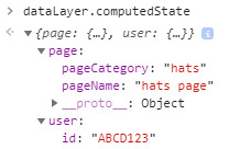
My first step is to create an SVG element that I can use as a base for the drawing. The picture below is an idea of where I want to get: a nice, scalable canvas with a detailed grid to guide my orientation on the plane. Part of the plan is to mold my canvas to a specific shape: a 100×100 square, to be precise. To get me there, 4 elements will need to come together: a base SVG shape, x and y axes, scales to transform the input accordingly to the window size, and grids across the square.
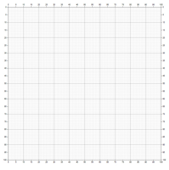
The first goal: create a 100×100 SVG canvas
The first thing I will do is making sure my SVG is scalable and works well on all resolutions. Here I used the viewBox property and panned it a bit to the top left to accommodate for the scales that I’m planning to add.
var w = 800;
var h = 800;
var svg = d3.select("div#container").append("svg")
.attr("preserveAspectRatio", "xMinYMin meet")
.attr("viewBox", "-20 -20 " + w + " " + h)
//this is to zoom out
//.attr("viewBox", "-20 -20 1600 1600")
.style("padding", 5)
.style("margin", 5);
Getting SVG right can be tricky. Especially if you, like me, have the innate ability to misunderstand things at the first sight. The first time I touched the viewBox property not only I badly misconfigured it, but it also took me a couple of hours to unlearn it.
The viewBox attribute is responsible for specifying the start (x, y) and the zoom (w, h) of an SVG. If you set the zoom properties to anything lower than the width and height of your page then it will zoom in. Anything bigger, it will zoom out. I found that zooming out is useful when I’m working on the whole composition, hence the commented out line: .attr(“viewBox”, “-20 -20 1600 1600”).
Scales, axes, and grids
Since my SVG can scale depending on the window resolution, I need everything else to scale with it: that includes both canvas elements like axes and the shapes I’m planning to draw later on. D3 takes care of linear scaling of data with the built-in function d3.scaleLinear() that takes an input domain (e.g. 0 to 100) and transforms it to a range of values (e.g. onto 0 to 200). In my case I want my input data to be translated to my current window’s height and width. I’ll point to those values in my scales’ range accessor. The viewBox function will then take care of scaling it elegantly. The input domain will be set to [0,100] for x, and [100,0] for y as I want to fit everything on a square that measures 100^2.
//PREPARE SCALES
var xScale = d3.scaleLinear()
//accepts
.domain([0, 100])
//outputs
.range([0, w]);
var yScale = d3.scaleLinear()
//accepts
.domain([0, 100])
//outputs
.range([0, h]);
The next elements I will draw are the axes and the grids. I don’t have the type of spacial imagination to feel comfortable on an abstract SVG plane. The constant need to calculate where to put my next point gives me anxiety. Take a bar chart: it would start at a point that has an x and a y, each bar has a certain height, so you’d subtract that height from the SVG’s height (otherwise the bars will be hanging from above like stalactites), then add to it a couple of more transformations. This has me lost in space. Axes give me reasonable comfort, but I thought with grid lines I could achieve maximum control over things.
My axes will surround the square I want to force the data points onto. The axes will run along every side of the square, with ticks every 5 steps of my (0, 100) range.
//PREPARE AXES
var xAxisBottom = d3.axisBottom(xScale).ticks(20);
var xAxisTop = d3.axisTop(xScale).ticks(20);
var yAxisLeft = d3.axisLeft(yScale).ticks(20);
var yAxisRight = d3.axisRight(yScale).ticks(20);
//DRAW AXES
svg.append("g")
.attr("class", "axis")
.attr("transform", "translate(0," + h + ")")
.call(xAxisBottom);
svg.append("g")
.attr("class", "axis")
.call(xAxisTop);
svg.append("g")
.attr("class", "axis")
.call(yAxisLeft);
svg.append("g")
.attr("class", "axis")
.attr("transform", "translate(" + w + ",0)")
.call(yAxisRight);
You will notice that I needed to move the bottom axis to the square’s bottom with the translate function – and the right axis to the right side of the square. translate can be used to move any object from its default or previously defined position. The orientation [Bottom|Top|Left|Right] chosen with d3.axis only defines the orientation of the ticks.
My canvas with the axes added looks like this. Happy times: the square is clearly visible.
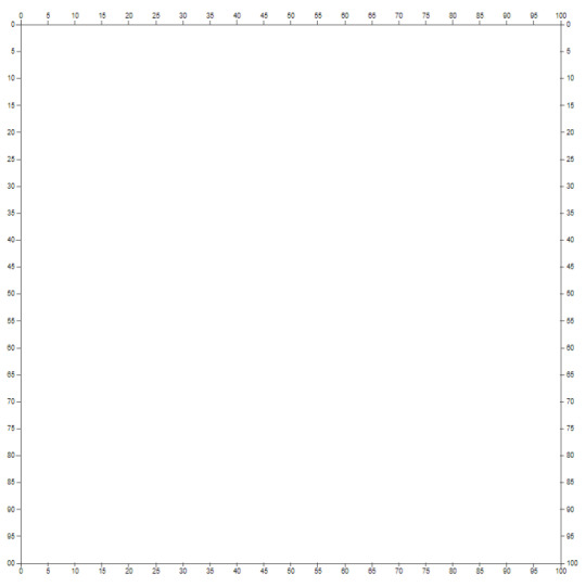
Second step: adding in the axes
The next step is to construct the grid lines. I decided that there will be a grid line crossing the square at every 10 points – that is my major grid. Every 1 point I will draw an auxiliary grid line, marked in the CSS with a lighter grey. Grids are constructed with the same function my axes used. The grids are in fact stretched ticks of an axis. See how I set their property to the square’s height and width.
//PREPARE GRIDS
//MAIN
var ygridlines = d3.axisTop()
.tickFormat("")
.tickSize(-h)
.ticks(10)
.scale(xScale);
var xgridlines = d3.axisLeft()
.tickFormat("")
.tickSize(-w)
.ticks(10)
.scale(yScale);
//MINOR
var ygridlinesmin = d3.axisTop()
.tickFormat("")
.tickSize(-h)
.ticks(100)
.scale(xScale);
var xgridlinesmin = d3.axisLeft()
.tickFormat("")
.tickSize(-w)
.ticks(100)
.scale(yScale);
//DRAW GRIDS
//MINOR GRID
svg.append("g")
.attr("class", "minor-grid")
.call(ygridlinesmin);
svg.append("g")
.attr("class", "minor-grid")
.call(xgridlinesmin);
//MAIN GRID
svg.append("g")
.attr("class", "main-grid")
.call(ygridlines);
svg.append("g")
.attr("class", "main-grid")
.call(xgridlines);
After the grids are plotted on the SVG, the base canvas is ready:

Fun shapes
It’s time to get to drawing – the fun part.
Drawing a rectangle is incredibly easy as D3 provides a pre-defined D3 shape, rect. A rect shape can be appended directly to the SVG. You need to give your shape a height, a width, and the starting coordinates. Then you pass it via our scaling functions (xScale and yScale, depending on whether something is on the x or y axis), and append it to the SVG.
var rect = svg.append("rect")
.attr("height",function(d){
return yScale(50);})
.attr("width", function(d){
return xScale(10);})
.attr("y",function(d){
return yScale(10);})
.attr("x",function(d){
return xScale(10);})
.attr("class", "rectangle");
This code plots a rectangle on my canvas:
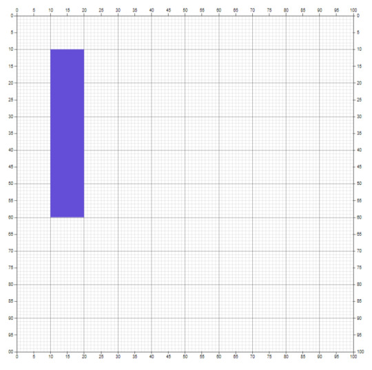
A purple rectangle is added
Drawing a line is not particularly difficult either, but it requires a bit of understanding how d3.line() function works. The function accepts an array of coordinates and draws a line through them. So the only thing we do is provide those points and pass them through the function and the appropriate scale. Note that my scales accept a domain of 0 to 100, so I had to adhere to it when defining the data points.
var lineGenerator = d3.line()
.x(function(d) { return xScale(d[0]) })
.y(function(d) { return yScale(d[1]) });
var points = [
[40, 30],
[50, 20],
[60, 13],
[70, 25],
[80, 10],
[90, 15]
];
var pathData = lineGenerator(points);
var freeline = svg.append("path")
.attr("class", "freeline")
.attr("d", function(d) { return pathData ; });
The line is plotted as expected:
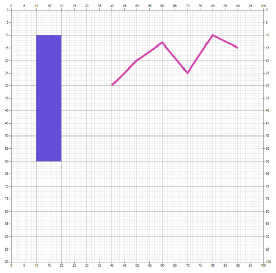
A pink line joins in
Drawing a radial shape has proven a bit complex. I recommend you take a look at my previous post Drawing radial shapes in D3.js to get a good grip on the function logic. Here I went with an area radial shape to be able to fill the shape up with color. While the drawing logic is the same as in the example of the d3.radialLine(), the syntax of the function is a tad different. The function d3.radialArea() asks for 3 inputs: the angle, the inner circle’s radius, and the outer circle’s radius. The outer circle corresponds with the outer border of the shape; the inner is the inner border. Here inner is set to 0, because I want to fully fill the shape.
var radialLineGenerator = d3.radialArea()
.innerRadius(function(d) {
return xScale(d[1])})
.outerRadius(function(d) {
return xScale(d[2])});
var radialpoints = [
[0, 0, 15],
[Math.PI * 0.2, 0, 6],
[Math.PI * 0.4, 0, 15],
[Math.PI * 0.6, 0, 6],
[Math.PI * 0.8, 0, 15],
[Math.PI * 1, 0, 6],
[Math.PI * 1.2, 0, 15],
[Math.PI * 1.4, 0, 6],
[Math.PI * 1.6, 0, 15],
[Math.PI * 1.8, 0, 6],
[Math.PI * 2, 0, 15]
];
var radialData = radialLineGenerator(radialpoints);
var radial = svg.append("path")
.attr("class", "freeradial")
.attr("d", radialData)
.attr("class", "radial")
.attr("transform", function(d) {
return "translate("+xScale(60)+","+yScale(60)+")"
});
This adds a green star to the canvas:
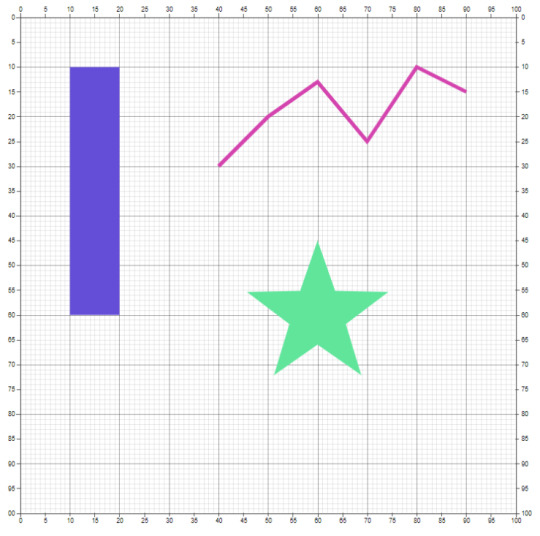
A green star completes the party
Here is my full code if you want to replicate the exercise:
shapes.html:
<!DOCTYPE html>
<html lang="en">
<head>
<meta charset="utf-8">
<title>Fun Shapes</title>
<script type="text/javascript" src="https://d3js.org/d3.v5.min.js"></script>
<link rel="stylesheet" type="text/css" href="shapes.css">
<style></style>
</head>
<body>
<div id="container" class="svg-container"></div>
<script type="text/javascript">
var w = 800;
var h = 800;
var svg = d3.select("div#container").append("svg")
.attr("preserveAspectRatio", "xMinYMin meet")
.attr("viewBox", "-20 -20 " + w + " " + h)
//this is to zoom out
//.attr("viewBox", "-20 -20 1600 1600")
.style("padding", 5)
.style("margin", 5);
//----------------CANVAS PREPARATION----------------//
//PREPARE SCALES
//PREPARE SCALES
var xScale = d3.scaleLinear()
//accepts
.domain([0, 100])
//outputs
.range([0, w]);
var yScale = d3.scaleLinear()
//accepts
.domain([0, 100])
//outputs
.range([0, h]);
//PREPARE AXES
var xAxisBottom = d3.axisBottom(xScale).ticks(20);
var xAxisTop = d3.axisTop(xScale).ticks(20);
var yAxisLeft = d3.axisLeft(yScale).ticks(20);
var yAxisRight = d3.axisRight(yScale).ticks(20);
//PREPARE GRIDS
//MAIN
var ygridlines = d3.axisTop()
.tickFormat("")
.tickSize(-h)
.ticks(10)
.scale(xScale);
var xgridlines = d3.axisLeft()
.tickFormat("")
.tickSize(-w)
.ticks(10)
.scale(yScale);
//MINOR
var ygridlinesmin = d3.axisTop()
.tickFormat("")
.tickSize(-h)
.ticks(100)
.scale(xScale);
var xgridlinesmin = d3.axisLeft()
.tickFormat("")
.tickSize(-w)
.ticks(100)
.scale(yScale);
//DRAW EVERYTHING
//LAYER BOTTOM UP
//MINOR GRID
svg.append("g")
.attr("class", "minor-grid")
.call(ygridlinesmin);
svg.append("g")
.attr("class", "minor-grid")
.call(xgridlinesmin);
//MAIN GRID
svg.append("g")
.attr("class", "main-grid")
.call(ygridlines);
svg.append("g")
.attr("class", "main-grid")
.call(xgridlines);
//AXES
svg.append("g")
.attr("class", "axis")
.attr("transform", "translate(0," + h + ")")
.call(xAxisBottom);
svg.append("g")
.attr("class", "axis")
.call(xAxisTop);
svg.append("g")
.attr("class", "axis")
.call(yAxisLeft);
svg.append("g")
.attr("class", "axis")
.attr("transform", "translate(" + w + ",0)")
.call(yAxisRight);
//----------------FUN SHAPES----------------//
//RECTANGLE
var rect = svg.append("rect")
.attr("height",function(d){
return yScale(50);})
.attr("width", function(d){
return xScale(10);})
.attr("y",function(d){
return yScale(10);})
.attr("x",function(d){
return xScale(10);})
.attr("class", "rectangle");
//LINE
var lineGenerator = d3.line()
.x(function(d) { return xScale(d[0]) })
.y(function(d) { return yScale(d[1]) });
var points = [
[40, 30],
[50, 20],
[60, 13],
[70, 25],
[80, 10],
[90, 15]
];
var pathData = lineGenerator(points);
var freeline = svg.append("path")
.attr("class", "freeline")
.attr("d", function(d) { return pathData ; });
//RADIAL SHAPE
var radialLineGenerator = d3.radialArea()
.innerRadius(function(d) {
return xScale(d[1])})
.outerRadius(function(d) {
return xScale(d[2])});
var radialpoints = [
[0, 0, 15],
[Math.PI * 0.2, 0, 6],
[Math.PI * 0.4, 0, 15],
[Math.PI * 0.6, 0, 6],
[Math.PI * 0.8, 0, 15],
[Math.PI * 1, 0, 6],
[Math.PI * 1.2, 0, 15],
[Math.PI * 1.4, 0, 6],
[Math.PI * 1.6, 0, 15],
[Math.PI * 1.8, 0, 6],
[Math.PI * 2, 0, 15]
];
var radialData = radialLineGenerator(radialpoints);
var radial = svg.append("path")
.attr("class", "freeradial")
.attr("d", radialData)
.attr("class", "radial")
.attr("transform", function(d) {
return "translate("+xScale(60)+","+yScale(60)+")"
});
</script>
</body>
</html>
shapes.css:
/* grids */
.minor-grid {
stroke: #cccccc;
stroke-width: 0.1;
shape-rendering: crispEdges;
}
.main-grid {
color: #212121;
stroke-width: 0.4;
shape-rendering: crispEdges;
}
/* ticks */
.axis line{
stroke: #3f3f3f;
shape-rendering: crispEdges;
}
/* contour */
.axis path {
stroke: #3f3f3f;
shape-rendering: crispEdges;
}
/* rectangle */
rect.rectangle {
fill: #644dd7;
}
/* line */
path.freeline {
stroke: #d444ae;
stroke-width: 6;
fill: none;
}
/* radial shape */
path.radial {
stroke: none;
fill: #60e59b;
}
I hope you enjoyed the post. As always, please point out any problems you see with this solution in the comments. In the next post I will go on more SVG adventures!
Follow @EveTheAnalyst
DataTau published first on DataTau
0 notes
Text
Advanced NLP with SpaCy
About this course
In this course, you'll learn how to use spaCy to build advanced natural language understanding systems, using both rule-based and machine learning approaches. I originally developed the content for DataCamp, but I wanted to make a free version so you don't have to sign up for their service. As a weekend project, I ended up putting together my own little app to present the exercises and content in a fun and interactive way.
About me

I'm Ines, and I'm one of the core developers of spaCy and the co-founder of Explosion. I specialise in applications and developer tools for AI, Machine Learning and Natural Language Processing technologies. I also really love building stuff for the web.
DataTau published first on DataTau
0 notes
Text
Train models and run notebooks on AWS cheaper and simpler than with SageMaker

Oleg Polosin
Sep 18, 2018
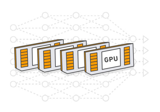

Spotty is a tool that drastically simplifies training of deep learning models on AWS.
Why will you ❤️ this tool?
it makes training on AWS GPU instances as simple as training on your local computer
it automatically manages all necessary AWS resources including AMIs, volumes, snapshots and SSH keys
it makes your model trainable on AWS by everyone with a couple of commands
it uses tmux to easily detach remote processes from SSH sessions
it saves you up to 70% of the costs by using AWS Spot Instances
To show how it works let’s take some non-trivial model and try to train it. I chose one of the implementations of Tacotron 2. It’s a speech synthesis system by Google.
Clone the repository of Tacotron 2 to your computer:
git clone https://github.com/Rayhane-mamah/Tacotron-2.git
Docker Image
Spotty trains models inside a Docker container. So we need to either find a publicly available Docker image that satisfies the model’s requirements or create a new Dockerfile with a proper environment.
This implementation of Tacotron uses Python 3 and TensorFlow, so we could use the official Tensorflow image from Docker Hub. But this image doesn’t satisfy all the requirements from the “requirements.txt” file. So we need to extend the image and install all necessary libraries on top of it.
Copy the “requirements.txt” file to the “docker/requirements-spotty.txt” file and create thedocker/Dockerfile.spotty file with the following content:

Here we’re extending the original TensorFlow image and installing all other requirements. This image will be built automatically when you start an instance.
Spotty Configuration File
Once we have the Dockerfile, we’re ready to write a Spotty configuration file. Create aspotty.yaml file in the root directory of your project.
Here you can find the full content of this file. It consists of 4 sections: project, container, instances, and scripts. Let’s look at them one by one.
Section 1: Project
This section contains the following parameters:
name: name of the project. This name will be used in the names of all AWS resources created by Spotty for this project. For example, it will be used as a prefix for EBS volumes, or in the name of the S3 bucket that helps to synchronize the project’s code with the instance.
syncFilters: synchronization filters. These filters will be used to skip some directories or files when synchronizing the project’s code with a running instance. In the example above we’re ignoring PyCharm configuration, Git files, Python cache files, and training data. Under the hood, Spotty is using these filters with the “aws s3 sync” command, so you can get more information about them here: Use of Exclude and Include Filter.
Section 2: Container
This section describes a Docker container for your project:
projectDir: a directory inside the container where the local project will be synchronized once an instance is started. Make sure that either it’s a subdirectory of a volume mount path (see below) or it exactly matches a volume mount path, otherwise, all remote changes to the project’s code will be lost once the instance is stopped.
volumeMounts: defines directories inside a container where EBS volumes should be mounted. EBS volumes themselves will be described in the instances section of the configuration file. Each element of this list describes one mount point, where the name parameter should match the corresponding EBS volume from the instance section (see below), and the mountPath parameter specifies a volume’s directory inside a container.
file: a path to the Dockerfile that we created before. The Docker image will be built automatically once the instance is started. As an alternative approach, you could build the image locally and push it to Docker Hub, then you can directly specify the image by its name using the image parameter instead of the file parameter.
ports: ports that should be exposed by the instance. In the example above we opened 2 ports: 6006 for TensorBoard and 8888 for Jupyter Notebook.
Read more about other container parameters in the documentation.
Section 3: Instances
This section describes a list of instances with their parameters. Each instance contains the following parameters:
name: name of the instance. This name will be used in the names of AWS resources that were created specifically for this instance. For example, EBS volumes and an EC2 instance itself. Also, this name can be used in the Spotty commands if you have more than one instance in the configuration file. For example, spotty start i1.
provider: a cloud provider for the instance. At the moment Spotty supports only “aws” provider (Amazon Web Services), but Google Cloud Platform will be supported in the near future as well.
parameters: parameters of the instance. They are specific to a cloud provider. See parameters for an AWS instance below.
AWS instance parameters:
region: AWS region where a Spot Instance should be launched.
instanceType: type of an EC2 instance. Read more about AWS GPU instances here.
volumes: a list of EBS volumes that should be attached to the instance. To have a volume attached to the container’s filesystem, the name parameter should match one of the volumeMounts names from the container section. See the description of an EBS volume parameters below.
dockerDataRoot: using this parameter we can change a directory where Docker stores all images including our built image. In the example above we make sure that it’s a directory on an attached EBS volume. So next time the image will not be rebuilt again, but just loaded from the Docker cache.
EBS volume parameters:
size: size of the volume in GB.
deletionPolicy: what to do with the volume once the instance is stopped using the spotty stop command. Possible values include: “create_snapshot” (default), “update_snapshot”, “retain” and “delete”. Read more in the documentation: Volumes and Deletion Policies.
mountDir: a directory where the volume will be mounted on the instance. By default, it will be mounted to the “/mnt/<ebs_volume_name>” directory. In the example above, we need to explicitly specify this directory for the “docker” volume, because we reuse this value in the dockerDataRoot parameter.
Read more about other AWS instance parameters in the documentation.
Section 4: Scripts
Scripts are optional but very useful. They can be run on the instance using the following command:
spotty run <SCRIPT_NAME>
For this project we’ve created 4 scripts:
preprocess: downloads the dataset and prepares it for training,
train: starts training,
tensorboard: runs TensorBoard on the port 6006,
jupyter: starts Jupyter Notebook server on the port 8888.
That’s it! The model is ready to be trained on AWS.
Spotty Installation
Requirements
Python ≥3.5
Installed and configured AWS CLI (see Installing the AWS Command Line Interface)
Installation
1. Install the Spotty using pip:
pip install -U spotty
2. Create an AMI with NVIDIA Docker. Run the following command from the root directory of your project (where the spotty.yaml file is located):
spotty aws create-ami
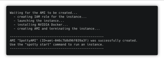

In several minutes you will have an AMI that can be used for all your projects within the AWS region.
Model Training
1. Start a Spot Instance with the Docker container:
spotty start
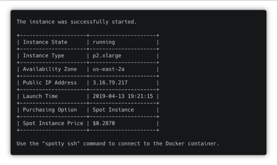

Once the instance is up and running, you will see its IP address. Use it to open TensorBoard and Jupyter Notebook later.
2. Download and preprocess the data for the Tacotron model. We already have a custom script in the configuration file to do that, just run:
spotty run preprocess
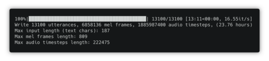

Once the data is processed, use the Ctrl + b, then x combination of keys to close the tmux pane.
3. Once the preprocessing is done, train the model. Run the “train” script:
spotty run train

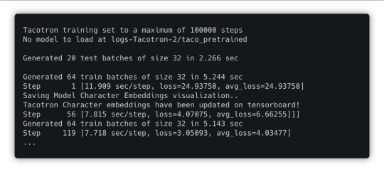
You can detach this SSH session using the Ctrl + b, then d combination of keys. The training process won’t be interrupted. To reattach that session, just run the spotty run train command again.
TensorBoard
Start TensorBoard using the “tensorboard” script:
spotty run tensorboard
TensorBoard will be running on the port 6006. You can detach the SSH session using the Ctrl + b, then d combination of keys, TensorBoard will still be running.
Jupyter Notebook
You also can start Jupyter Notebook using the “jupyter” script:
spotty run jupyter
Jupyter Notebook will be running on the port 8888. Open it using the instance IP address and the token that you will see in the command output.
Download Checkpoints
If you need to download checkpoints or any other files from the running instance to your local machine, just use the download command:
spotty download -f 'logs-Tacotron-2/taco_pretrained/*'
SSH Connection
To connect to the running Docker container via SSH, use the following command:
spotty ssh
It uses a tmux session, so you can always detach it using the Ctrl + b, then d combination of keys and attach that session later using the spotty ssh command again.
Don’t forget to stop the instance once you are done! Use the following command:
spotty stop
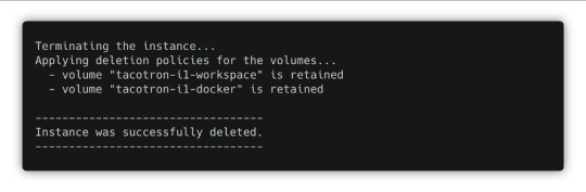

In the example above we used the “retain” deletion policy for our volumes, so Spotty will just terminate the instance and won’t touch the volumes. But it could automatically create snapshots if we would use “create_snapshot” or “update_snapshot” deletion policies.
Conclusion
Using Spotty is a convenient way to train deep learning models on AWS Spot Instances. It will save you not just up to 70% of the costs, but also a lot of time on setting up an environment for your models and notebooks. Once you have a Spotty configuration for your model, everyone can train it with a couple of commands.
If you enjoyed this post, please star the project on GitHub, click the 👏 button and share this post with your friends.
DataTau published first on DataTau
0 notes
Text
A Gentle Introduction to Padding and Stride for Convolutional Neural Networks
The convolutional layer in convolutional neural networks systematically applies filters to an input and creates output feature maps.
Although the convolutional layer is very simple, it is capable of achieving sophisticated and impressive results. Nevertheless, it can be challenging to develop an intuition for how the shape of the filters impacts the shape of the output feature map and how related configuration hyperparameters such as padding and stride should be configured.
In this tutorial, you will discover an intuition for filter size, the need for padding, and stride in convolutional neural networks.
After completing this tutorial, you will know:
How filter size or kernel size impacts the shape of the output feature map.
How the filter size creates a border effect in the feature map and how it can be overcome with padding.
How the stride of the filter on the input image can be used to downsample the size of the output feature map.
Let’s get started.
A Gentle Introduction to Padding and Stride for Convolutional Neural Networks
Photo by Red~Star, some rights reserved.
Tutorial Overview
This tutorial is divided into five parts; they are:
Convolutional Layer
Problem of Border Effects
Effect of Filter Size (Kernel Size)
Fix the Border Effect Problem With Padding
Downsample Input With Stride
Want Results with Deep Learning for Computer Vision?
Take my free 7-day email crash course now (with sample code).
Click to sign-up and also get a free PDF Ebook version of the course.
Download Your FREE Mini-Course
Convolutional Layer
In a convolutional neural network, a convolutional layer is responsible for the systematic application of one or more filters to an input.
The multiplication of the filter to the input image results in a single output. The input is typically three-dimensional images (e.g. rows, columns and channels), and in turn, the filters are also three-dimensional with the same number of channels and fewer rows and columns than the input image. As such, the filter is repeatedly applied to each part of the input image, resulting in a two-dimensional output map of activations, called a feature map.
Keras provides an implementation of the convolutional layer called a Conv2D.
It requires that you specify the expected shape of the input images in terms of rows (height), columns (width), and channels (depth) or [rows, columns, channels].
The filter contains the weights that must be learned during the training of the layer. The filter weights represent the structure or feature that the filter will detect and the strength of the activation indicates the degree to which the feature was detected.
The layer requires that both the number of filters be specified and that the shape of the filters be specified.
We can demonstrate this with a small example. In this example, we define a single input image or sample that has one channel and is an eight pixel by eight pixel square with all 0 values and a two-pixel wide vertical line in the center.
# define input data data = [[0, 0, 0, 1, 1, 0, 0, 0], [0, 0, 0, 1, 1, 0, 0, 0], [0, 0, 0, 1, 1, 0, 0, 0], [0, 0, 0, 1, 1, 0, 0, 0], [0, 0, 0, 1, 1, 0, 0, 0], [0, 0, 0, 1, 1, 0, 0, 0], [0, 0, 0, 1, 1, 0, 0, 0], [0, 0, 0, 1, 1, 0, 0, 0]] data = asarray(data) data = data.reshape(1, 8, 8, 1)
Next, we can define a model that expects input samples to have the shape (8, 8, 1) and has a single hidden convolutional layer with a single filter with the shape of three pixels by three pixels.
# create model model = Sequential() model.add(Conv2D(1, (3,3), input_shape=(8, 8, 1))) # summarize model model.summary()
The filter is initialized with random weights as part of the initialization of the model. We will overwrite the random weights and hard code our own 3×3 filter that will detect vertical lines.
That is the filter will strongly activate when it detects a vertical line and weakly activate when it does not. We expect that by applying this filter across the input image, the output feature map will show that the vertical line was detected.
# define a vertical line detector detector = [[[[0]],[[1]],[[0]]], [[[0]],[[1]],[[0]]], [[[0]],[[1]],[[0]]]] weights = [asarray(detector), asarray([0.0])] # store the weights in the model model.set_weights(weights)
Next, we can apply the filter to our input image by calling the predict() function on the model.
# apply filter to input data yhat = model.predict(data)
The result is a four-dimensional output with one batch, a given number of rows and columns, and one filter, or [batch, rows, columns, filters].
We can print the activations in the single feature map to confirm that the line was detected.
# enumerate rows for r in range(yhat.shape[1]): # print each column in the row print([yhat[0,r,c,0] for c in range(yhat.shape[2])])
Tying all of this together, the complete example is listed below.
# example of using a single convolutional layer from numpy import asarray from keras.models import Sequential from keras.layers import Conv2D # define input data data = [[0, 0, 0, 1, 1, 0, 0, 0], [0, 0, 0, 1, 1, 0, 0, 0], [0, 0, 0, 1, 1, 0, 0, 0], [0, 0, 0, 1, 1, 0, 0, 0], [0, 0, 0, 1, 1, 0, 0, 0], [0, 0, 0, 1, 1, 0, 0, 0], [0, 0, 0, 1, 1, 0, 0, 0], [0, 0, 0, 1, 1, 0, 0, 0]] data = asarray(data) data = data.reshape(1, 8, 8, 1) # create model model = Sequential() model.add(Conv2D(1, (3,3), input_shape=(8, 8, 1))) # summarize model model.summary() # define a vertical line detector detector = [[[[0]],[[1]],[[0]]], [[[0]],[[1]],[[0]]], [[[0]],[[1]],[[0]]]] weights = [asarray(detector), asarray([0.0])] # store the weights in the model model.set_weights(weights) # apply filter to input data yhat = model.predict(data) # enumerate rows for r in range(yhat.shape[1]): # print each column in the row print([yhat[0,r,c,0] for c in range(yhat.shape[2])])
Running the example first summarizes the structure of the model.
Of note is that the single hidden convolutional layer will take the 8×8 pixel input image and will produce a feature map with the dimensions of 6×6. We will go into why this is the case in the next section.
We can also see that the layer has 10 parameters, that is nine weights for the filter (3×3) and one weight for the bias.
Finally, the feature map is printed. We can see from reviewing the numbers in the 6×6 matrix that indeed the manually specified filter detected the vertical line in the middle of our input image.
_________________________________________________________________ Layer (type) Output Shape Param # ================================================================= conv2d_1 (Conv2D) (None, 6, 6, 1) 10 ================================================================= Total params: 10 Trainable params: 10 Non-trainable params: 0 _________________________________________________________________ [0.0, 0.0, 3.0, 3.0, 0.0, 0.0] [0.0, 0.0, 3.0, 3.0, 0.0, 0.0] [0.0, 0.0, 3.0, 3.0, 0.0, 0.0] [0.0, 0.0, 3.0, 3.0, 0.0, 0.0] [0.0, 0.0, 3.0, 3.0, 0.0, 0.0] [0.0, 0.0, 3.0, 3.0, 0.0, 0.0]
Problem of Border Effects
In the previous section, we defined a single filter with the size of three pixels high and three pixels wide (rows, columns).
We saw that the application of the 3×3 filter, referred to as the kernel size in Keras, to the 8×8 input image resulted in a feature map with the size of 6×6.
That is, the input image with 64 pixels was reduced to a feature map with 36 pixels. Where did the other 28 pixels go?
The filter is applied systematically to the input image. It starts at the top left corner of the image and is moved from left to right one pixel column at a time until the edge of the filter reaches the edge of the image.
For a 3×3 pixel filter applied to a 8×8 input image, we can see that it can only be applied six times, resulting in the width of six in the output feature map.
For example, let’s work through each of the six patches of the input image (left) dot product (“.” operator) the filter (right):
0, 0, 0 0, 1, 0 0, 0, 0 . 0, 1, 0 = 0 0, 0, 0 0, 1, 0
Moved right one pixel:
0, 0, 1 0, 1, 0 0, 0, 1 . 0, 1, 0 = 0 0, 0, 1 0, 1, 0
Moved right one pixel:
0, 1, 1 0, 1, 0 0, 1, 1 . 0, 1, 0 = 3 0, 1, 1 0, 1, 0
Moved right one pixel:
1, 1, 0 0, 1, 0 1, 1, 0 . 0, 1, 0 = 3 1, 1, 0 0, 1, 0
Moved right one pixel:
1, 0, 0 0, 1, 0 1, 0, 0 . 0, 1, 0 = 0 1, 0, 0 0, 1, 0
Moved right one pixel:
0, 0, 0 0, 1, 0 0, 0, 0 . 0, 1, 0 = 0 0, 0, 0 0, 1, 0
That gives us the first row and each column of the output feature map:
0.0, 0.0, 3.0, 3.0, 0.0, 0.0
The reduction in the size of the input to the feature map is referred to as border effects. It is caused by the interaction of the filter with the border of the image.
This is often not a problem for large images and small filters but can be a problem with small images. It can also become a problem once a number of convolutional layers are stacked.
For example, below is the same model updated to have two stacked convolutional layers.
This means that a 3×3 filter is applied to the 8×8 input image to result in a 6×6 feature map as in the previous section. A 3×3 filter is then applied to the 6×6 feature map.
# example of stacked convolutional layers from keras.models import Sequential from keras.layers import Conv2D # create model model = Sequential() model.add(Conv2D(1, (3,3), input_shape=(8, 8, 1))) model.add(Conv2D(1, (3,3))) # summarize model model.summary()
Running the example summarizes the shape of the output from each layer.
We can see that the application of filters to the feature map output of the first layer, in turn, results in a smaller 4×4 feature map.
This can become a problem as we develop very deep convolutional neural network models with tens or hundreds of layers. We will simply run out of data in our feature maps upon which to operate.
_________________________________________________________________ Layer (type) Output Shape Param # ================================================================= conv2d_1 (Conv2D) (None, 6, 6, 1) 10 _________________________________________________________________ conv2d_2 (Conv2D) (None, 4, 4, 1) 10 ================================================================= Total params: 20 Trainable params: 20 Non-trainable params: 0 _________________________________________________________________
Effect of Filter Size (Kernel Size)
Different sized filters will detect different sized features in the input image and, in turn, will result in differently sized feature maps.
It is common to use 3×3 sized filters, and perhaps 5×5 or even 7×7 sized filters, for larger input images.
For example, below is an example of the model with a single filter updated to use a filter size of 5×5 pixels.
# example of a convolutional layer from keras.models import Sequential from keras.layers import Conv2D # create model model = Sequential() model.add(Conv2D(1, (5,5), input_shape=(8, 8, 1))) # summarize model model.summary()
Running the example demonstrates that the 5×5 filter can only be applied to the 8×8 input image 4 times, resulting in a 4×4 feature map output.
_________________________________________________________________ Layer (type) Output Shape Param # ================================================================= conv2d_1 (Conv2D) (None, 4, 4, 1) 26 ================================================================= Total params: 26 Trainable params: 26 Non-trainable params: 0 _________________________________________________________________
It may help to further develop the intuition of the relationship between filter size and the output feature map to look at two extreme cases.
The first is a filter with the size of 1×1 pixels.
# example of a convolutional layer from keras.models import Sequential from keras.layers import Conv2D # create model model = Sequential() model.add(Conv2D(1, (1,1), input_shape=(8, 8, 1))) # summarize model model.summary()
Running the example demonstrates that the output feature map has the same size as the input, specifically 8×8. This is because the filter only has a single weight (and a bias).
_________________________________________________________________ Layer (type) Output Shape Param # ================================================================= conv2d_1 (Conv2D) (None, 8, 8, 1) 2 ================================================================= Total params: 2 Trainable params: 2 Non-trainable params: 0 _________________________________________________________________
The other extreme is a filter with the same size as the input, in this case, 8×8 pixels.
# example of a convolutional layer from keras.models import Sequential from keras.layers import Conv2D # create model model = Sequential() model.add(Conv2D(1, (8,8), input_shape=(8, 8, 1))) # summarize model model.summary()
Running the example, we can see that, as you might expect, there is one weight for each pixel in the input image (64 + 1 for the bias) and that the output is a feature map with a single pixel.
_________________________________________________________________ Layer (type) Output Shape Param # ================================================================= conv2d_1 (Conv2D) (None, 1, 1, 1) 65 ================================================================= Total params: 65 Trainable params: 65 Non-trainable params: 0 _________________________________________________________________
Now that we are familiar with the effect of filter sizes on the size of the resulting feature map, let’s look at how we can stop losing pixels.
Fix the Border Effect Problem With Padding
By default, a filter starts at the left of the image with the left-hand side of the filter sitting on the far left pixels of the image. The filter is then stepped across the image one column at a time until the right-hand side of the filter is sitting on the far right pixels of the image.
An alternative approach to applying a filter to an image is to ensure that each pixel in the image is given an opportunity to be at the center of the filter.
By default, this is not the case, as the pixels on the edge of the input are only ever exposed to the edge of the filter. By starting the filter outside the frame of the image, it gives the pixels on the border of the image more of an opportunity for interacting with the filter, more of an opportunity for features to be detected by the filter, and in turn, an output feature map that has the same shape as the input image.
For example, in the case of applying a 3×3 filter to the 8×8 input image, we can add a border of one pixel around the outside of the image. This has the effect of artificially creating a 10×10 input image. When the 3×3 filter is applied, it results in an 8×8 feature map. The added pixel values could have the value zero value that has no effect with the dot product operation when the filter is applied.
x, x, x 0, 1, 0 x, 0, 0 . 0, 1, 0 = 0 x, 0, 0 0, 1, 0
The addition of pixels to the edge of the image is called padding.
In Keras, this is specified via the “padding” argument on the Conv2D layer, which has the default value of ‘valid‘ (no padding). This means that the filter is applied only to valid ways to the input.
The ‘padding‘ value of ‘same‘ calculates and adds the padding required to the input image (or feature map) to ensure that the output has the same shape as the input.
The example below adds padding to the convolutional layer in our worked example.
# example a convolutional layer with padding from keras.models import Sequential from keras.layers import Conv2D # create model model = Sequential() model.add(Conv2D(1, (3,3), padding='same', input_shape=(8, 8, 1))) # summarize model model.summary()
Running the example demonstrates that the shape of the output feature map is the same as the input image: that the padding had the desired effect.
_________________________________________________________________ Layer (type) Output Shape Param # ================================================================= conv2d_1 (Conv2D) (None, 8, 8, 1) 10 ================================================================= Total params: 10 Trainable params: 10 Non-trainable params: 0 _________________________________________________________________
The addition of padding allows the development of very deep models in such a way that the feature maps do not dwindle away to nothing.
The example below demonstrates this with three stacked convolutional layers.
# example a deep cnn with padding from keras.models import Sequential from keras.layers import Conv2D # create model model = Sequential() model.add(Conv2D(1, (3,3), padding='same', input_shape=(8, 8, 1))) model.add(Conv2D(1, (3,3), padding='same')) model.add(Conv2D(1, (3,3), padding='same')) # summarize model model.summary()
Running the example, we can see that with the addition of padding, the shape of the output feature maps remains fixed at 8×8 even three layers deep.
_________________________________________________________________ Layer (type) Output Shape Param # ================================================================= conv2d_1 (Conv2D) (None, 8, 8, 1) 10 _________________________________________________________________ conv2d_2 (Conv2D) (None, 8, 8, 1) 10 _________________________________________________________________ conv2d_3 (Conv2D) (None, 8, 8, 1) 10 ================================================================= Total params: 30 Trainable params: 30 Non-trainable params: 0 _________________________________________________________________
Downsample Input With Stride
The filter is moved across the image left to right, top to bottom, with a one-pixel column change on the horizontal movements, then a one-pixel row change on the vertical movements.
The amount of movement between applications of the filter to the input image is referred to as the stride, and it is almost always symmetrical in height and width dimensions.
The default stride or strides in two dimensions is (1,1) for the height and the width movement, performed when needed. And this default works well in most cases.
The stride can be changed, which has an effect both on how the filter is applied to the image and, in turn, the size of the resulting feature map.
For example, the stride can be changed to (2,2). This has the effect of moving the filter two pixels left for each horizontal movement of the filter and two pixels down for each vertical movement of the filter when creating the feature map.
We can demonstrate this with an example using the 8×8 image with a vertical line (left) dot product (“.” operator) with the vertical line filter (right) with a stride of two pixels:
0, 0, 0 0, 1, 0 0, 0, 0 . 0, 1, 0 = 0 0, 0, 0 0, 1, 0
Moved right two pixels:
0, 1, 1 0, 1, 0 0, 1, 1 . 0, 1, 0 = 3 0, 1, 1 0, 1, 0
Moved right two pixels:
1, 0, 0 0, 1, 0 1, 0, 0 . 0, 1, 0 = 0 1, 0, 0 0, 1, 0
We can see that there are only three valid applications of the 3×3 filters to the 8×8 input image with a stride of two. This will be the same in the vertical dimension.
This has the effect of applying the filter in such a way that the normal feature map output (6×6) is down-sampled so that the size of each dimension is reduced by half (3×3), resulting in 1/4 the number of pixels (36 pixels down to 9).
The stride can be specified in Keras on the Conv2D layer via the ‘stride‘ argument and specified as a tuple with height and width.
The example demonstrates the application of our manual vertical line filter on the 8×8 input image with a convolutional layer that has a stride of two.
# example of vertical line filter with a stride of 2 from numpy import asarray from keras.models import Sequential from keras.layers import Conv2D # define input data data = [[0, 0, 0, 1, 1, 0, 0, 0], [0, 0, 0, 1, 1, 0, 0, 0], [0, 0, 0, 1, 1, 0, 0, 0], [0, 0, 0, 1, 1, 0, 0, 0], [0, 0, 0, 1, 1, 0, 0, 0], [0, 0, 0, 1, 1, 0, 0, 0], [0, 0, 0, 1, 1, 0, 0, 0], [0, 0, 0, 1, 1, 0, 0, 0]] data = asarray(data) data = data.reshape(1, 8, 8, 1) # create model model = Sequential() model.add(Conv2D(1, (3,3), strides=(2, 2), input_shape=(8, 8, 1))) # summarize model model.summary() # define a vertical line detector detector = [[[[0]],[[1]],[[0]]], [[[0]],[[1]],[[0]]], [[[0]],[[1]],[[0]]]] weights = [asarray(detector), asarray([0.0])] # store the weights in the model model.set_weights(weights) # apply filter to input data yhat = model.predict(data) # enumerate rows for r in range(yhat.shape[1]): # print each column in the row print([yhat[0,r,c,0] for c in range(yhat.shape[2])])
Running the example, we can see from the summary of the model that the shape of the output feature map will be 3×3.
Applying the handcrafted filter to the input image and printing the resulting activation feature map, we can see that, indeed, the filter still detected the vertical line, and can represent this finding with less information.
Downsampling may be desirable in some cases where deeper knowledge of the filters used in the model or of the model architecture allows for some compression in the resulting feature maps.
_________________________________________________________________ Layer (type) Output Shape Param # ================================================================= conv2d_1 (Conv2D) (None, 3, 3, 1) 10 ================================================================= Total params: 10 Trainable params: 10 Non-trainable params: 0 _________________________________________________________________ [0.0, 3.0, 0.0] [0.0, 3.0, 0.0] [0.0, 3.0, 0.0]
Further Reading
This section provides more resources on the topic if you are looking to go deeper.
Posts
Crash Course in Convolutional Neural Networks for Machine Learning
Books
Chapter 9: Convolutional Networks, Deep Learning, 2016.
Chapter 5: Deep Learning for Computer Vision, Deep Learning with Python, 2017.
API
Keras Convolutional Layers API
Summary
In this tutorial, you discovered an intuition for filter size, the need for padding, and stride in convolutional neural networks.
Specifically, you learned:
How filter size or kernel size impacts the shape of the output feature map.
How the filter size creates a border effect in the feature map and how it can be overcome with padding.
How the stride of the filter on the input image can be used to downsample the size of the output feature map.
Do you have any questions?
Ask your questions in the comments below and I will do my best to answer.
The post A Gentle Introduction to Padding and Stride for Convolutional Neural Networks appeared first on Machine Learning Mastery.
Machine Learning Mastery published first on Machine Learning Mastery
0 notes
Text
Physics of Everday Life
Based on Scott's review, I read through Stephen Pinker's Enlightenment Now. I can't top Scott's exposition of the book, but it is pretty incredible how far humanity has gone when you step back to look at the big picture.
One line intrigued me, one that Pinker credits to a book called The Big Picture by Sean Carroll
The laws of physics underlying everyday life (that is excluding extreme values of energy and gravitation like black holes, dark matter and the Big Bang) are completely known.
Hasn't this statement almost always been true, in the sense that the leading minds would make this claim at many times in history. The ancient Greeks probably believed they understood physics that underlies everyday life. So did physicists after Newton. Life back then not today. My everyday life involves using a GPS device that requires understanding relativistic effects and computer chips that needed other scientific advances.
Is it possible we could do more in everyday life if we knew more physics? I'd certainly use a teleporter in everyday life.
And is the statement even true today? We all use public key cryptography, even to read this blog. It's not completely clear if we understand the physics enough to know how or if large-scale quantum computers capable of breaking those systems can be built.
Everday life is relative.
Computational Complexity published first on Computational Complexity
0 notes
Text
“Please, explain.” Interpretability of black-box machine learning models
In February 2019 Polish government added an amendment to a banking law that gives a customer a right to receive an explanation in case of a negative credit decision. It’s one of the direct consequences of implementing GDPR in EU. This means that a bank needs to be able to explain why the loan wasn’t granted if the decision process was automatic.
In October 2018 world headlines reported about Amazon AI recruiting tool that favored men. Amazon’s model was trained on biased data that were skewed towards male candidates. It has built rules that penalized résumés that included the word “women’s”.
Consequences of not understanding models’ predictions
What is common for the two examples above is that both models in the banking industry and the one built by Amazon are very complex tools, so-called black-box classifiers, that don’t offer straightforward and human-interpretable decision rules.
Financial institutions will have to invest in model interpretability research if they want to continue using ML-based solutions. And they probably will, because such algorithms are more accurate in predicting credit risk. Amazon on the other hand, could have saved a lot of money and bad press if the model was properly validated and understood.
Why now? Trends in data modeling.
Machine learning has continued to stay on the top of Gartner’s Hype Cycle since 2014, to be replaced by the Deep Learning (a form of ML) in 2018 suggesting the adoption hasn’t reached its peak yet.
Machine learning growth is predicted to further accelerate. Based on the report by Univa 96% of the companies are expected to use ML in production in the next 2 years.
The reasons behind this are: widespread data collection, availability of vast computation resources and active open-source community. ML adoption growth is accompanied by the increase in ML-interpretability research driven by regulations like GDPR, EU’s “right to explain”, concerns about safety (medicine, autonomous vehicles), reproducibility and bias or end-users expectations (debug the model to improve it or learn something new about the studied subject).
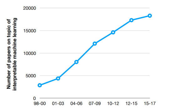
Source: http://people.csail.mit.edu/beenkim/papers/BeenK_FinaleDV_ICML2017_tutorial.pdf
Black-box algorithms interpretability possibilities
As data scientists, we should be able to provide an explanation to end users about how a model works. However, this not necessarily means understanding every piece of the model or generating a set of decision rules.
There could also be a case where this is not required:
problem is well studied,
model results has no consequences,
understanding the model by the end-user could pose a risk of gaming the system.
If we look at the results from the Kaggle’s Machine Learning and Data Science Survey from 2018, around 60% of respondents think they could explain most of machine learning models (some models were still hard to explain for them). The most common approach used to ML understanding is analyzing model features by looking at feature importance and feature correlations.
Feature importance analysis offers first good insights into what the model is learning and what factors might be important. However, this technique can be unreliable if features are correlated. It can provide good insights only if model variables are interpretable. For many GBMs libraries it’s fairly easy to generate feature importance plots.
In the case of Deep Learning situation is much more complicated. When using neural networks you could look at weights, as they contain the information about the input, but the information is compressed. What’s more, you can only analyze the connections on the first level, since on further levels it’s too complicated.
No wonder that when in 2016 LIME (Local Interpretable Model-Interpretable Explanations) paper was presented at NIPS conference it had a huge impact. The idea behind LIME is to locally approximate a black-box model with an easier to understand white-box model constructed on interpretable input data. It has proven great results providing interpretation for image classification and text. However, for tabular data, it’s difficult to find interpretable features and their local interpretation might be misleading.
LIME is implemented in Python (lime and Skater) and R (lime package and iml package, live package) and is very easy to use.
Another promising idea is SHAP (Shapley Additive Explanations). It’s based on game theory. It assumes that features are players, models are coalitions and Shapley values tell how to fairly distribute the “payout” among the features. This technique distributes the effects fairly, is easy to use and offers visually compelling implementation.
DALEX package (Descriptive Machine Learning Explanations) available in R offers a set of tools that help to understand how complex models are working. Using DALEX you can create model explainer and inspect it visually e.g. breakdown plots. You might also be interested in DrWhy.Ai which is developed by the same group of researchers as DALEX.
Practical use cases
Detecting objects on the pictures
Image recognition is already widely used, among others in autonomous cars to detect if cars, traffic lights etc. are on the picture, in wildlife conservation to detect if a certain animal is in the picture or in the insurance to detect flooding of crops.
We will use the “Husky vs Wolf example” from the original LIME paper to illustrate the importance of model interpretation. The classifier task was to identify if a wolf was on the picture or not. It falsely misclassified Siberian Husky as a wolf. Thanks to LIME researchers were able to identify what areas of the pictures were important for the model. It turned out that if the picture contains snow it is classified as a wolf.
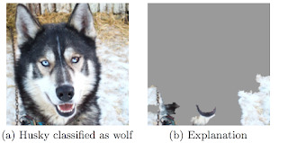
Source: LIME paper
The algorithm was using the background of the picture and totally ignoring animal characteristics. The model should look at the animal eyes instead. Thanks to this discovery it was possible to fix the model and extend the training examples to prevent the reasoning snow = wolf.
Classification as decision support system
Intensive Care Unit of Amsterdam UMC wants predict the probabilities of patient’s readmission and/or mortality at the moment of discharge. The goal is to help doctors pick the right moment to move the patient from ICU. If the doctor understands what the model is doing is more likely to use it’s recommendation in making the final judgement.
In order to demonstrate how such model can be interpreted using LIME, we can have a look at the example from another study that aims to do early prediction of the mortality at the ICU. Random Forest model (a black-box model) is used to predict mortality status and lime package is used to locally explain the prediction score for every patient.
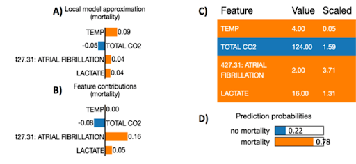
Source: https://www.researchgate.net/publication/309551203_Machine_Learning_Model_Interpretability_for_Precision_Medicine
A patient from the selected example has high death probability (78%). The model features that contribute to mortality are higher counts of atrial fibrillation and higher lactate level, which is consistent with current medical understanding.
Humans and machines – a perfect match
In order to achieve success in building an interpretable AI we need to combine data science knowledge, algorithms and end users expertise. Data science work doesn’t finish after creating the model. It’s an iterative, usually long process with feedback loops provided by the experts, making sure the outcome is solid and understandable by humans.
We strongly believe that by combining humans expertise and machines performance we can obtain the best conclusion: improve machine results and overcome human gut-feel bias.
Please enable JavaScript to view the comments powered by Disqus.
DataTau published first on DataTau
0 notes
Text
Keeping master green at scale
Keeping master green at scale Ananthanarayanan et al., EuroSys’19
This paper provides a fascinating look at a key part of Uber’s software delivery machine. With a monorepo, and many thousands of engineers concurrently committing changes, keeping the build green, and keeping commit-to-live latencies low, is a major challenge.
This paper introduces a change management system called SubmitQueue that is responsible for continuous integration of changes into the mainline at scale while always keeping the mainline green.
The challenge: build fails at scale
Each individual submitted change will have passed all local tests, but when you put large numbers of concurrent changes together conflicts can still happen. Finding out what’s gone wrong is a tedious and error-prone task often requiring human intervention. Meanwhile, new features are blocked from rolling out.
So the goal is to keep it green:
…the monorepo mainline needs to remain green at all times. A mainline is called green if all build steps (e.g., compilation, unit tests, UI tests) can successfully execute for every commit point in the history. Keeping the mainline green allows developers to (i) instantly release new features from any commit point in the mainline, (ii) roll back to any previously committed change, and not necessarily to the last working version, and (iii) always develop against the most recent and healthy version of the monorepo.
Here’s 9 months of data for the Uber iOS and Android repos, showing the probability of conflicts as the number of concurrent changes increases:
At ‘only’ 16 concurrent and potentially conflicting changes, there’s a 40% chance of a problem. Thus, “despite all efforts to minimize mainline breakages, it is very likely that the mainline experiences daily breakages due to the sheer volume of everyday code changes committed to a big monorepo.”
And that’s exactly what Uber saw. Here’s a one week view of the iOS mainline prior to the introduction of SubmitQueue. The mainline was green only 52% of the time.
(Since the introduction of SubmitQueue over a year ago, mainlines have remained green at all times).
To keep the mainline green we need to totally order changes and only apply patches to mainline HEAD if all build steps succeed.
The simplest solution to keep the mainline green is to enqueue every change that gets submitted to the system. A change at the head of the queue gets committed into the mainline if its build steps succeed. For instance, the rustproject uses this technique to ensure that the mainline remains healthy all the time. This approach does not scale as the number of changes grows. For instance, with a thousand changes per day, where each change takes 30 minutes to pass all build steps, the turnaround time of the last enqueued change will be over 20 days.
20 day turnarounds clearly is not going to lead to a high performing organisation! One possible solution to reduce the latency is batching changes, but then we’re back at the problem of conflicts and complex manual resolution if we’re not careful. Another tactic is optimistic execution – given enough compute we can start builds in parallel on, with the assumption that all pending changes submitted will succeed. This approach suffers from high failure rates and turnaround times still though as failure of a change can abort many optimistically executing builds.
SubmitQueue
Uber’s solution to these challenges is SubmitQueue.
SubmitQueue guarantees an always green mainline by providing the illusion of a single queue where every change gets enqueued, performs all its build steps, and ultimately gets merged with the mainline branch if all build steps succeed.
Developers create changes, which pending a review process are packaged into a revision. Revisions are submitted to the SubmitQueue for integration into the monorepo.
SubmitQueue’s planner engine orchestrates executions of ending changes.
In order to scale to thousands of changes per day while ensuring serializability, the planner engine speculates on outcomes of pending changes using a speculation engine, and executes their corresponding builds in parallel by using a build controller.
The planner periodically asks the speculation engine for the builds most likely to succeed. The speculation engine in turn uses a probabilistic model to compute the likelihood of a given build passing. At each epoch the planner schedules execution of the selected builds and stops execution of any currently running builds not included in the new schedule. Once it is safe to do so, the planner commits change patches to the monorepo. When distributing work among worker nodes, the planner tries to ensure a uniform distribution. To this end, it keep a history of build steps performed together with their average build durations.
The key challenge is to determine which set of builds we need to run in parallel, in order to improve turnaround time and throughput, while ensuring an always green mainline. To this end, the speculation engine builds a binary decision tree, called a speculation tree, annotated with prediction probabilities for each edge.
The model selects builds based on their predicted value – which is a combination of likelihood of success and change priority (e.g. , security patches may have higher values). In the current implementation, all builds are given the same priority (benefit) value.
When we include independent changes in the mix, the speculation tree can become a speculation graph. This enables independent changes to be committed in parallel. To determine independence, we need to know if changes conflict with each other.
In order to build a conflict graph among pending changes, the conflict analyzer relies on the build system. A build system partitions the code into smaller entities called targets… Roughly speaking, two changes conflict if they both affect a common set of build targets.
Every build target is associated with a unique target hash that represents its current state (a bit like a Merkle tree, this is the result of combining the hashes of all the inputs to the build of that target).
Predicting success
We trained our success prediction models in a supervised manner using logistic regression. We selected historical changes that went through SubmitQueue along with their final results for this purpose. We then extracted around 100 handpicked features.
The trained model achieved 97% accuracy. The features with the highest positive correlation scores were:
The number of successful speculations so far
Revision and revert test plans included as part of the submission
The number of initial tests that succeeded before submitting a change
The strongest negative correlations were with the number of failed speculations, and the number of times changes were submitted to a revision.
We also note that while developer features such as the developer name had high predictive power, the correlation varied based on different developers.
Evaluation
Taken in isolation, an iOS or Android build at Uber takes around 30-60 minutes:
When considering concurrent changes, and given an Oracle able to make perfect predictions, the turnaround times for builds looks like this:
(Each plot line shows a different number of changes per hour coming into the system).
With n changes per hour, and n worker nodes available, SubmitQueue can achieve a turnaround time with 1.2x of the Oracle.
Future work
The current version of SubmitQueue respects the order in which changes are submitted to the system. Thus small changes can be backed up behind larger ones. Future work will include re-ordering of non-independent changes to improve throughput. Another optimisation to be explored is batching independent changes expected to succeed together before running their build steps. This will enable Uber to make trade-offs between cost and turnaround time.
the morning paper published first on the morning paper
0 notes
Text
Instacart Data Science Interviews
More than 50% of American families order grocery via Instacart.

Vimarsh Karbhari
Apr 17
Instacart can predict the realtime availability of 200 million grocery items in US and Canada stores. By the end of 2018, 80% of American households will be able to use Instacart. Their teams made data science interesting by using Deep Learning with Emojis. The tech at Instacart blog shares the interesting experiments and Instacart’s journey through Data Science. After going through their blog, it should become very evident that Instacart has one of the best Data Science teams and Data Science problems for a Data professional to work on.

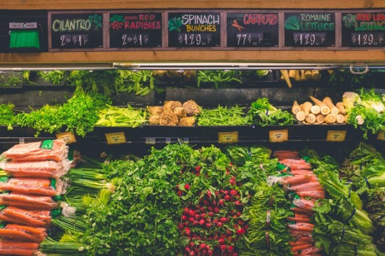
Photo by NeONBRAND on Unsplash
Interview Process
The interview process is pretty straightforward. It starts with a data challenge, followed by a technical phone interview. After you pass these two, there is a round of technical and culture fit interviews on-site. The interviews are short and targeted and provide you a good insight into the job and the teams you’ll work with at Instacart.
Important Reading
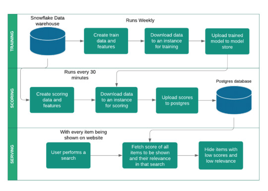

Scoring:(Source) Realtime availability of 200 million grocery
Space, time and Groceries: Instacart tech
Instacart Anytime: Data Science at Instacart
How Instacart delivers on time: Using quantile regression
Data Science Related Interview Questions
When an item isn’t available, what algorithm should we use to replace it?
How would you staff the team based on delivery data?
What other products or revenue opportunities will arise from Instacart’s data?
Write a script to format data in a text file.
Estimate the demand and supply
How might you have optimized parameters for this model differently?
How would you tune a random forest?
Given a OLTP system which tracks the sales of items with order processing, returns and shipping, create a data warehouse model to find gross sales, net sales and gross sales by product.
Given a movie database, identify whether a movie has well defined genre.
How should we solve our supply / demand problems at Instacart?
Reflecting on the Questions
The data science team at Instacart publishes blog articles regularly Engineering Instacart blog. At Instacart, data drives product decisions which reflects in their questions. The questions are aimed to get information on how you will meld within the existing team and if you can think in terms of the problems they are trying to solve. The scale of the items they catalog is huge. Something as day to day as groceries are looked from the purview of data science is interesting. A good knack to solve problems related to logistics and scale can surely land you a job with the largest grocery catalog in the world!
Subscribe to our Acing AI newsletter, I promise not to spam and its FREE!
Acing AI Newsletter — Revue
Acing AI Newsletter — Reducing the entropy in Data Science and AI. Aimed to help people get into AI and Data Science by…www.getrevue.co
Thanks for reading! 😊 If you enjoyed it, test how many times can you hit 👏 in 5 seconds. It’s great cardio for your fingers AND will help other people see the story.
The sole motivation of this blog article is to learn about Instacart and its technologies helping people to get into it. All data is sourced from online public sources. I aim to make this a living document, so any updates and suggested changes can always be included. Please provide relevant feedback.
DataTau published first on DataTau
0 notes
Text
Teaching rigorous distributed systems with efficient model checking
Teaching rigorous distributed systems with efficient model checking Michael et al., EuroSys’19
On the surface you might think today’s paper selection an odd pick. It describes the labs environment, DSLabs, developed at the University of Washington to accompany a course in distributed systems. During the ten week course, students implement four different assignments: an exactly-once RPC protocol; a primary-backup system; Paxos; and a scalable, transactional key-value storage system. 175 undergraduates a year currently go through this course. Enabling students to build running performant versions of all of those systems in the time available is one challenge. Testing and grading their solutions is another!
Although we added tests to catch specific issues as we learned of them, we found it difficult to keep up with the diversity of possible student errors.
What I like about the paper is that (a) the DSLabs framework and all assignments are available in open source, and it looks like it would be a lot of fun to play with, and (b) the challenges students have to face in building reliable, testable, distributed systems under time pressure look pretty much like the challenges many practitioners have to face to me! So by focusing on what it takes to help students be successful in this context, we can also derive some inspiration for building systems in the wild too.
DSLabs combines traditional testing with model checking:
Faced with the challenges of building robust distributed systems and the inadequacies of other methodologies, both academic research and industry have increasingly turned to model checking to validate system correctness. Model checking overcomes the weakness of ad hoc testing by systematically exploring all possible executions, but without the high labor cost of formal verification.
At this point you might think of turning to TLA+. However, it’s difficult to master this environment and learn core distributed systems concepts in a single term, and moreover a model checked TLA+ specification still has to then be implemented in some language. Hence the DSLabs framework integrates model checking into a holistic distributed systems development environment (based on Java as the implementation language – it would be neat to see a Rust version!).
This paper introduces DSLabs, a framework for writing, testing, model checking, running, and debugging distributed systems, along with a sequence of assignments written to use the framework.
In the core programming model, students provide implementations of Node subclasses which specify the behaviour of individual nodes in their distributed systems. Each node runs in a single threaded event loop. The interface is pretty straightforward:
The only thing that looks slightly odd on first glance in that interface is the set timer method that takes a min duration and max duration. To make things easily testable, all handlers are required to be deterministic. But hang on a minute you may say, isn’t a little randomness very useful in constructing distributed systems? Yes it is! In the DSLabs environment the only allowable randomness is encapsulated in that timer call, which will expire the timer at a random time between the min and max parameter values.
Clients are also implemented as Nodes. Worker drivers are provided by the tutors and execute a pre-determined workload using clients written by students.
The networking model is asynchronous (allowing out of order, dropped, delayed, and duplicated messages), the failure model is crash-stop.
Testing and model checking
One of the goals of DSLabs is for students to create runnable distributed systems. We would like students to consider the performance characteristics of their systems, and our tests check that their designs attain reasonable run-time performance.
It’s hard to exhaustively test a distributed system with traditional testing techniques. So DSLabs also uses model checking. Consider the lab exercise to implement Paxos. One common implementation error (i.e., one observed being made by many students) is to accept a value being proposed without also checking the proposal number (see full explanation in §3.1 of the paper).
While this bug could cause a violation of linearizability, witnessing such a violation would be rare… In light of our goal of providing a thorough suite of tests, not being able to find a common bug like this one is problematic! On the other hand, model checking can find this bug reliably.
So we need an approachable model checking solution that doesn’t come with a steep learning curve, and can find common bugs in a timely fashion. These twin requirements led DSLabs to incorporate its own lightweight model checking solution. In addition, another lesson here is that once we accept model checking is necessary, we need to design systems that are amenable to model checking.
I would be nice if students did not have to take model checking into consideration (aside from ensuring their systems meet the basic requirements…). If this were true, the model checking tests we provide would simply be better tests which reliably caught distributed systems bugs. However, systems design decisions can have a large impact on the performance of the model checker, and thus its ability to find bugs within a reasonable amount of time.
The heuristic advice given to students is as follows:
Favour simplicity above all else
Do not keep or send unnecessary state
Explore performance optimisations, but not at the expense of significant added complexity
Consider the number of events it takes for your system to make progress from any state; ensure that number is reasonably close to the minimum.
Luckily, code that is readily model checkable usually corresponds to the kind of code we want students to write — code that is as simple as possible with respect to its state graph.
As we saw earlier, the DSLabs model checker requires deterministic handlers. It collapses equivalent states to avoid wasting work during model checking (in this case, based on equals and hashCode methods generated for students by Project Lombok). Even then, the state space can be huge (e.g. exponential in n, where n is the number of steps). The model checker needs to provide timely feedback rather than having it run for hours and hours every time. So DSLabs uses two basic strategies to focus the search in the areas most likely to be fruitful:
We’d like to know how deep into the graph we need to explore. One way to do this is to ensure the model checker has gone deep enough for the system to be able to make progress. So we can search for states in which progress has been made, and assume that this depth is also enough as a first pass to find not only states where we have made good progress, but also states where we take ‘bad’ actions.
There will still remain places where the model checker needs to probe deeper. For example, the Paxos bug alluded to earlier takes a minimum of 36 steps to trigger. DSLabs uses a guided search strategy here, using knowledge about each system’s specification to guide the model checker’s search to more interesting and error-prone parts of the state space. Prunes are predicates telling the model checker which states not to expand. Punctuated search first looks for states satisfying some intermediate constraint, and then restarts a (deeper) search from there.
DSLabs post-processes failing traces to present them in the easiest to understand form possible for students, with events laid out in causal order wherever possible.
A visual debugger/system explorer
DSLabs also includes a visual debugger called Oddity, which can be used to explore system behaviour. Oddity will also start automatically when the model checker finds an invariant violation. It looks like this:
Teaching distributed systems using DSLabs
The following table shows the LOC count for the reference implementations of each assignment in DSLabs.
A solution implemented in TLA+ would likely be smaller, but only modestly so, at the expense of students needing to learn a completely new language.
The table above also shows wall clock time for running the tests (including model checking). The DSLabs test suite can give useful feedback in six minutes or less (on the reference solutions), fast enough to be part of an iterative development process.
This supports our goal of giving students timely feedback… Prior to adding model checking, it was common for students to find bugs in their Paxos implementation only when they tried to use that implementation in a later lab. By catching student errors more quickly , we reduce the amount of rework needed.
For the Paxos bug described earlier, the DSLabs guided search can find it in 18 seconds. As a comparison, an unguided search took an average of 12 hours to do so.
The hardest part of the class for many students is learning to think about their code as inherently distributed. This in turn requires thinking about the invariants maintained by the system over all possible event sequences simultaneously. It highlights a case where students, perhaps trained on good TDD practices (do students get taught that these days??) and used to taking small incremental steps, fail to appreciate the need for some degree of up-front design. (Of course, we never make that mistake in industry;) ).
Students often march though test cases incrementally, fixing problems only once they occur. A particular student tried this for the primary-backup assignment and got stuck: the fix for a problem found by one test would often break the solution for previous tests. The student found he could find a version to pass each of the tests, just not the same version. After we encouraged him to start over with a clean design that met all of the criteria simultaneously, he was able to quickly converge on a solution.
The model checking was a big help here as it surfaced bugs students may not have realised were latent in their code.
The last word
Using the DSLabs framework and assignments, we have successfully guided hundreds of students through the process of building a fault-tolerant, scalable, distributed key–value store. Furthermore, these student-built systems are actually runnable, rather than mere specifications; they can be deployed in a fully distributed fashion and can achieve considerable performance.
I’ll leave you with another reminder that if you want to play with it, the labs environment and assignments can all be found on GitHub…
the morning paper published first on the morning paper
0 notes
Text
A Gentle Introduction to Convolutional Layers for Deep Learning Neural Networks
Convolution and the convolutional layer are the major building blocks used in convolutional neural networks.
A convolution is the simple application of a filter to an input that results in an activation. Repeated application of the same filter to an input results in a map of activations called a feature map, indicating the locations and strength of a detected feature in an input, such as an image.
The innovation of convolutional neural networks is the ability to automatically learn a large number of filters in parallel specific to a training dataset under the constraints of a specific predictive modeling problem, such as image classification. The result is highly specific features that can be detected anywhere on input images.
In this tutorial, you will discover how convolutions work in the convolutional neural network.
After completing this tutorial, you will know:
Convolutional neural networks apply a filter to an input to create a feature map that summarizes the presence of detected features in the input.
Filters can be handcrafted, such as line detectors, but the innovation of convolutional neural networks is to learn the filters during training in the context of a specific prediction problem.
How to calculate the feature map for one- and two-dimensional convolutional layers in a convolutional neural network.
Let’s get started.
A Gentle Introduction to Convolutional Layers for Deep Learning Neural Networks
Photo by mendhak, some rights reserved.
Tutorial Overview
This tutorial is divided into four parts; they are:
Convolution in Convolutional Neural Networks
Convolution in Computer Vision
Power of Learned Filters
Worked Example of Convolutional Layers
Want Results with Deep Learning for Computer Vision?
Take my free 7-day email crash course now (with sample code).
Click to sign-up and also get a free PDF Ebook version of the course.
Download Your FREE Mini-Course
Convolution in Convolutional Neural Networks
The convolutional neural network, or CNN for short, is a specialized type of neural network model designed for working with two-dimensional image data, although they can be used with one-dimensional and three-dimensional data.
Central to the convolutional neural network is the convolutional layer that gives the network its name. This layer performs an operation called a “convolution“.
In the context of a convolutional neural network, a convolution is a linear operation that involves the multiplication of a set of weights with the input, much like a traditional neural network. Given that the technique was designed for two-dimensional input, the multiplication is performed between an array of input data and a two-dimensional array of weights, called a filter or a kernel.
The filter is smaller than the input data and the type of multiplication applied between a filter-sized patch of the input and the filter is a dot product. A dot product is the element-wise multiplication between the filter-sized patch of the input and filter, which is then summed, always resulting in a single value. Because it results in a single value, the operation is often referred to as the “scalar product“.
Using a filter smaller than the input is intentional as it allows the same filter (set of weights) to be multiplied by the input array multiple times at different points on the input. Specifically, the filter is applied systematically to each overlapping part or filter-sized patch of the input data, left to right, top to bottom.
This systematic application of the same filter across an image is a powerful idea. If the filter is designed to detect a specific type of feature in the input, then the application of that filter systematically across the entire input image allows the filter an opportunity to discover that feature anywhere in the image. This capability is commonly referred to as translation invariance, e.g. the general interest in whether the feature is present rather than where it was present.
Invariance to local translation can be a very useful property if we care more about whether some feature is present than exactly where it is. For example, when determining whether an image contains a face, we need not know the location of the eyes with pixel-perfect accuracy, we just need to know that there is an eye on the left side of the face and an eye on the right side of the face.
— Page 342, Deep Learning, 2016.
The output from multiplying the filter with the input array one time is a single value. As the filter is applied multiple times to the input array, the result is a two-dimensional array of output values that represent a filtering of the input. As such, the two-dimensional output array from this operation is called a “feature map“.
Once a feature map is created, we can pass each value in the feature map through a nonlinearity, such as a ReLU, much like we do for the outputs of a fully connected layer.
Example of a Filter Applied to a Two-Dimensional Input to Create a Feature Map
If you come from a digital signal processing field or related area of mathematics, you may understand the convolution operation on a matrix as something different. Specifically, the filter (kernel) is flipped prior to being applied to the input. Technically, the convolution as described in the use of convolutional neural networks is actually a “cross-correlation”. Nevertheless, in deep learning, it is referred to as a “convolution” operation.
Many machine learning libraries implement cross-correlation but call it convolution.
— Page 333, Deep Learning, 2016.
In summary, we have a input, such as an image of pixel values, and we have a filter, which is a set of weights, and the filter is systematically applied to the input data to create a feature map.
Convolution in Computer Vision
The idea of applying the convolutional operation to image data is not new or unique to convolutional neural networks; it is a common technique used in computer vision.
Historically, filters were designed by hand by computer vision experts, which were then applied to an image to result in a feature map or output from applying the filter then makes the analysis of the image easier in some way.
For example, below is a hand crafted 3×3 element filter for detecting vertical lines:
0.0, 1.0, 0.0 0.0, 1.0, 0.0 0.0, 1.0, 0.0
Applying this filter to an image will result in a feature map that only contains vertical lines. It is a vertical line detector.
You can see this from the weight values in the filter; any pixels values in the center vertical line will be positively activated and any on either side will be negatively activated. Dragging this filter systematically across pixel values in an image can only highlight vertical line pixels.
A horizontal line detector could also be created and also applied to the image, for example:
0.0, 0.0, 0.0 1.0, 1.0, 1.0 0.0, 0.0, 0.0
Combining the results from both filters, e.g. combining both feature maps, will result in all of the lines in an image being highlighted.
A suite of tens or even hundreds of other small filters can be designed to detect other features in the image.
The innovation of using the convolution operation in a neural network is that the values of the filter are weights to be learned during the training of the network.
The network will learn what types of features to extract from the input. Specifically, training under stochastic gradient descent, the network is forced to learn to extract features from the image that minimize the loss for the specific task the network is being trained to solve, e.g. extract features that are the most useful for classifying images as dogs or cats.
In this context, you can see that this is a powerful idea.
Power of Learned Filters
Learning a single filter specific to a machine learning task is a powerful technique.
Yet, convolutional neural networks achieve much more in practice.
Multiple Filters
Convolutional neural networks do not learn a single filter; they, in fact, learn multiple features in parallel for a given input.
For example, it is common for a convolutional layer to learn from 32 to 512 filters in parallel for a given input.
This gives the model 32, or even 512, different ways of extracting features from an input, or many different ways of both “learning to see” and after training, many different ways of “seeing” the input data.
This diversity allows specialization, e.g. not just lines, but the specific lines seen in your specific training data.
Multiple Channels
Color images have multiple channels, typically one for each color channel, such as red, green, and blue.
From a data perspective, that means that a single image provided as input to the model is, in fact, three images.
A filter must always have the same number of channels as the input, often referred to as “depth“. If an input image has 3 channels (e.g. a depth of 3), then a filter applied to that image must also have 3 channels (e.g. a depth of 3). In this case, a 3×3 filter would in fact be 3x3x3 or [3, 3, 3] for rows, columns, and depth. Regardless of the depth of the input and depth of the filter, the filter is applied to the input using a dot product operation which results in a single value.
This means that if a convolutional layer has 32 filters, these 32 filters are not just two-dimensional for the two-dimensional image input, but are also three-dimensional, having specific filter weights for each of the three channels. Yet, each filter results in a single feature map. Which means that the depth of the output of applying the convolutional layer with 32 filters is 32 for the 32 feature maps created.
Multiple Layers
Convolutional layers are not only applied to input data, e.g. raw pixel values, but they can also be applied to the output of other layers.
The stacking of convolutional layers allows a hierarchical decomposition of the input.
Consider that the filters that operate directly on the raw pixel values will learn to extract low-level features, such as lines.
The filters that operate on the output of the first line layers may extract features that are combinations of lower-level features, such as features that comprise multiple lines to express shapes.
This process continues until very deep layers are extracting faces, animals, houses, and so on.
This is exactly what we see in practice. The abstraction of features to high and higher orders as the depth of the network is increased.
Worked Example of Convolutional Layers
The Keras deep learning library provides a suite of convolutional layers.
We can better understand the convolution operation by looking at some worked examples with contrived data and handcrafted filters.
In this section, we’ll look at both a one-dimensional convolutional layer and a two-dimensional convolutional layer example to both make the convolution operation concrete and provide a worked example of using the Keras layers.
Example of 1D Convolutional Layer
We can define a one-dimensional input that has eight elements all with the value of 0.0, with a two element bump in the middle with the values 1.0.
[0, 0, 0, 1, 1, 0, 0, 0]
The input to Keras must be three dimensional for a 1D convolutional layer.
The first dimension refers to each input sample; in this case, we only have one sample. The second dimension refers to the length of each sample; in this case, the length is eight. The third dimension refers to the number of channels in each sample; in this case, we only have a single channel.
Therefore, the shape of the input array will be [1, 8, 1].
# define input data data = asarray([0, 0, 0, 1, 1, 0, 0, 0]) data = data.reshape(1, 8, 1)
We will define a model that expects input samples to have the shape [8, 1].
The model will have a single filter with the shape of 3, or three elements wide. Keras refers to the shape of the filter as the kernel_size.
# create model model = Sequential() model.add(Conv1D(1, 3, input_shape=(8, 1)))
By default, the filters in a convolutional layer are initialized with random weights. In this contrived example, we will manually specify the weights for the single filter. We will define a filter that is capable of detecting bumps, that is a high input value surrounded by low input values, as we defined in our input example.
The three element filter we will define looks as follows:
[0, 1, 0]
The convolutional layer also has a bias input value that also requires a weight that we will set to zero.
Therefore, we can force the weights of our one-dimensional convolutional layer to use our handcrafted filter as follows:
# define a vertical line detector weights = [asarray([[[0]],[[1]],[[0]]]), asarray([0.0])] # store the weights in the model model.set_weights(weights)
The weights must be specified in a three-dimensional structure, in terms of rows, columns, and channels. The filter has a single row, three columns, and one channel.
We can retrieve the weights and confirm that they were set correctly.
# confirm they were stored print(model.get_weights())
Finally, we can apply the single filter to our input data.
We can achieve this by calling the predict() function on the model. This will return the feature map directly: that is the output of applying the filter systematically across the input sequence.
# apply filter to input data yhat = model.predict(data) print(yhat)
Tying all of this together, the complete example is listed below.
# example of calculation 1d convolutions from numpy import asarray from keras.models import Sequential from keras.layers import Conv1D # define input data data = asarray([0, 0, 0, 1, 1, 0, 0, 0]) data = data.reshape(1, 8, 1) # create model model = Sequential() model.add(Conv1D(1, 3, input_shape=(8, 1))) # define a vertical line detector weights = [asarray([[[0]],[[1]],[[0]]]), asarray([0.0])] # store the weights in the model model.set_weights(weights) # confirm they were stored print(model.get_weights()) # apply filter to input data yhat = model.predict(data) print(yhat)
Running the example first prints the weights of the network; that is the confirmation that our handcrafted filter was set in the model as we expected.
Next, the filter is applied to the input pattern and the feature map is calculated and displayed. We can see from the values of the feature map that the bump was detected correctly.
[array([[[0.]], [[1.]], [[0.]]], dtype=float32), array([0.], dtype=float32)] [[[0.] [0.] [1.] [1.] [0.] [0.]]]
Let’s take a closer look at what happened here.
Recall that the input is an eight element vector with the values: [0, 0, 0, 1, 1, 0, 0, 0].
First, the three-element filter [0, 1, 0] was applied to the first three inputs of the input [0, 0, 0] by calculating the dot product (“.” operator), which resulted in a single output value in the feature map of zero.
Recall that a dot product is the sum of the element-wise multiplications, or here it is (0 x 0) + (1 x 0) + (0 x 0) = 0. In NumPy, this can be implemented manually as:
from numpy import asarray print(asarray([0, 1, 0]).dot(asarray([0, 0, 0])))
In our manual example, this is as follows:
[0, 1, 0] . [0, 0, 0] = 0
The filter was then moved along one element of the input sequence and the process was repeated; specifically, the same filter was applied to the input sequence at indexes 1, 2, and 3, which also resulted in a zero output in the feature map.
[0, 1, 0] . [0, 0, 1] = 0
We are being systematic, so again, the filter is moved along one more element of the input and applied to the input at indexes 2, 3, and 4. This time the output is a value of one in the feature map. We detected the feature and activated appropriately.
[0, 1, 0] . [0, 1, 1] = 1
The process is repeated until we calculate the entire feature map.
[0, 0, 1, 1, 0, 0]
Note that the feature map has six elements, whereas our input has eight elements. This is an artefact of how the filter was applied to the input sequence. There are other ways to apply the filter to the input sequence that changes the shape of the resulting feature map, such as padding, but we will not discuss these methods in this post.
You can imagine that with different inputs, we may detect the feature with more or less intensity, and with different weights in the filter, that we would detect different features in the input sequence.
Example of 2D Convolutional Layer
We can expand the bump detection example in the previous section to a vertical line detector in a two-dimensional image.
Again, we can constrain the input, in this case to a square 8×8 pixel input image with a single channel (e.g. grayscale) with a single vertical line in the middle.
[0, 0, 0, 1, 1, 0, 0, 0] [0, 0, 0, 1, 1, 0, 0, 0] [0, 0, 0, 1, 1, 0, 0, 0] [0, 0, 0, 1, 1, 0, 0, 0] [0, 0, 0, 1, 1, 0, 0, 0] [0, 0, 0, 1, 1, 0, 0, 0] [0, 0, 0, 1, 1, 0, 0, 0] [0, 0, 0, 1, 1, 0, 0, 0]
The input to a Conv2D layer must be four-dimensional.
The first dimension defines the samples; in this case, there is only a single sample. The second dimension defines the number of rows; in this case, eight. The third dimension defines the number of columns, again eight in this case, and finally the number of channels, which is one in this case.
Therefore, the input must have the four-dimensional shape [samples, columns, rows, channels] or [1, 8, 8, 1] in this case.
# define input data data = [[0, 0, 0, 1, 1, 0, 0, 0], [0, 0, 0, 1, 1, 0, 0, 0], [0, 0, 0, 1, 1, 0, 0, 0], [0, 0, 0, 1, 1, 0, 0, 0], [0, 0, 0, 1, 1, 0, 0, 0], [0, 0, 0, 1, 1, 0, 0, 0], [0, 0, 0, 1, 1, 0, 0, 0], [0, 0, 0, 1, 1, 0, 0, 0]] data = asarray(data) data = data.reshape(1, 8, 8, 1)
We will define the Conv2D with a single filter as we did in the previous section with the Conv1D example.
The filter will be two-dimensional and square with the shape 3×3. The layer will expect input samples to have the shape [columns, rows, channels] or [8,8,1].
# create model model = Sequential() model.add(Conv2D(1, (3,3), input_shape=(8, 8, 1)))
We will define a vertical line detector filter to detect the single vertical line in our input data.
The filter looks as follows:
0, 1, 0 0, 1, 0 0, 1, 0
We can implement this as follows:
# define a vertical line detector detector = [[[[0]],[[1]],[[0]]], [[[0]],[[1]],[[0]]], [[[0]],[[1]],[[0]]]] weights = [asarray(detector), asarray([0.0])] # store the weights in the model model.set_weights(weights) # confirm they were stored print(model.get_weights())
Finally, we will apply the filter to the input image, which will result in a feature map that we would expect to show the detection of the vertical line in the input image.
# apply filter to input data yhat = model.predict(data)
The shape of the feature map output will be four-dimensional with the shape [batch, rows, columns, filters]. We will be performing a single batch and we have a single filter (one filter and one input channel), therefore the output shape is [1, ?, ?, 1]. We can pretty-print the content of the single feature map as follows:
for r in range(yhat.shape[1]): # print each column in the row print([yhat[0,r,c,0] for c in range(yhat.shape[2])])
Tying all of this together, the complete example is listed below.
# example of calculation 2d convolutions from numpy import asarray from keras.models import Sequential from keras.layers import Conv2D # define input data data = [[0, 0, 0, 1, 1, 0, 0, 0], [0, 0, 0, 1, 1, 0, 0, 0], [0, 0, 0, 1, 1, 0, 0, 0], [0, 0, 0, 1, 1, 0, 0, 0], [0, 0, 0, 1, 1, 0, 0, 0], [0, 0, 0, 1, 1, 0, 0, 0], [0, 0, 0, 1, 1, 0, 0, 0], [0, 0, 0, 1, 1, 0, 0, 0]] data = asarray(data) data = data.reshape(1, 8, 8, 1) # create model model = Sequential() model.add(Conv2D(1, (3,3), input_shape=(8, 8, 1))) # define a vertical line detector detector = [[[[0]],[[1]],[[0]]], [[[0]],[[1]],[[0]]], [[[0]],[[1]],[[0]]]] weights = [asarray(detector), asarray([0.0])] # store the weights in the model model.set_weights(weights) # confirm they were stored print(model.get_weights()) # apply filter to input data yhat = model.predict(data) for r in range(yhat.shape[1]): # print each column in the row print([yhat[0,r,c,0] for c in range(yhat.shape[2])])
Running the example first confirms that the handcrafted filter was correctly defined in the layer weights
Next, the calculated feature map is printed. We can see from the scale of the numbers that indeed the filter has detected the single vertical line with strong activation in the middle of the feature map.
[array([[[[0.]], [[1.]], [[0.]]], [[[0.]], [[1.]], [[0.]]], [[[0.]], [[1.]], [[0.]]]], dtype=float32), array([0.], dtype=float32)] [0.0, 0.0, 3.0, 3.0, 0.0, 0.0] [0.0, 0.0, 3.0, 3.0, 0.0, 0.0] [0.0, 0.0, 3.0, 3.0, 0.0, 0.0] [0.0, 0.0, 3.0, 3.0, 0.0, 0.0] [0.0, 0.0, 3.0, 3.0, 0.0, 0.0] [0.0, 0.0, 3.0, 3.0, 0.0, 0.0]
Let’s take a closer look at what was calculated.
First, the filter was applied to the top left corner of the image, or an image patch of 3×3 elements. Technically, the image patch is three dimensional with a single channel, and the filter has the same dimensions. We cannot implement this in NumPy using the dot() function, instead, we must use the tensordot() function so we can appropriately sum across all dimensions, for example:
from numpy import asarray from numpy import tensordot m1 = asarray([[0, 1, 0], [0, 1, 0], [0, 1, 0]]) m2 = asarray([[0, 0, 0], [0, 0, 0], [0, 0, 0]]) print(tensordot(m1, m2))
This calculation results in a single output value of 0.0, e.g., the feature was not detected. This gives us the first element in the top-left corner of the feature map.
Manually, this would be as follows:
0, 1, 0 0, 0, 0 0, 1, 0 . 0, 0, 0 = 0 0, 1, 0 0, 0, 0
The filter is moved along one column to the left and the process is repeated. Again, the feature is not detected.
0, 1, 0 0, 0, 1 0, 1, 0 . 0, 0, 1 = 0 0, 1, 0 0, 0, 1
One more move to the left to the next column and the feature is detected for the first time, resulting in a strong activation.
0, 1, 0 0, 1, 1 0, 1, 0 . 0, 1, 1 = 3 0, 1, 0 0, 1, 1
This process is repeated until the edge of the filter rests against the edge or final column of the input image. This gives the last element in the first full row of the feature map.
[0.0, 0.0, 3.0, 3.0, 0.0, 0.0]
The filter then moves down one row and back to the first column and the process is related from left to right to give the second row of the feature map. And on until the bottom of the filter rests on the bottom or last row of the input image.
Again, as with the previous section, we can see that the feature map is a 6×6 matrix, smaller than the 8×8 input image because of the limitations of how the filter can be applied to the input image.
Further Reading
This section provides more resources on the topic if you are looking to go deeper.
Posts
Crash Course in Convolutional Neural Networks for Machine Learning
Books
Chapter 9: Convolutional Networks, Deep Learning, 2016.
Chapter 5: Deep Learning for Computer Vision, Deep Learning with Python, 2017.
API
Keras Convolutional Layers API
numpy.asarray API
Summary
In this tutorial, you discovered how convolutions work in the convolutional neural network.
Specifically, you learned:
Convolutional neural networks apply a filter to an input to create a feature map that summarizes the presence of detected features in the input.
Filters can be handcrafted, such as line detectors, but the innovation of convolutional neural networks is to learn the filters during training in the context of a specific prediction problem.
How to calculate the feature map for one- and two-dimensional convolutional layers in a convolutional neural network.
Do you have any questions?
Ask your questions in the comments below and I will do my best to answer.
The post A Gentle Introduction to Convolutional Layers for Deep Learning Neural Networks appeared first on Machine Learning Mastery.
Machine Learning Mastery published first on Machine Learning Mastery
0 notes