oggistat

[oggistat]

Last Assignment

Good night! This is the last assignment of the course. I’ve really struggled to create a bivariate categorical graph, and I found out that there was a categorical variable that I was thinking it was numeric. Thus, I had to analyze alcohol consumption and smoking. Here’s the program:

@author: Bruno Oggioni Moura """

import pandas import numpy import seaborn import matplotlib.pyplot as plt

Data = pandas.read_csv('nesarc_pds.csv', low_memory=False)

# To avoid errors during runtime pandas.set_option('display.float_format', lambda x:'%f'%x)

#Setting variables to numeric Data['S2AQ8A'] = pandas.to_numeric(Data['S2AQ8A']) Data['S2AQ8B'] = pandas.to_numeric(Data['S2AQ8B']) Data['S2AQ10'] = pandas.to_numeric(Data['S2AQ10']) Data['S2BQ1A1'] = pandas.to_numeric(Data['S2BQ1A1']) Data['S2BQ1A9B'] = pandas.to_numeric(Data['S2BQ1A9B'])

#Subset sub1=Data[(Data['AGE']>=21)] sub2=sub1.copy()

sub2["S2AQ8A"] = sub2["S2AQ8A"].astype('category')

sub2["TAB12MDX"] = pandas.to_numeric(sub2['TAB12MDX'])

#Univariate categorical bar graph seaborn.countplot(x="S2AQ8A", data=sub2) plt.xlabel('How often drink alcohol past 12 months') plt.title('Alcohol consumption past 12 months')

# Bivariate categorical graph seaborn.catplot(x='S2AQ8A', y='TAB12MDX', data=sub2, kind="bar", ci=None) plt.xlabel('How often drink alcohol past 12 months') plt.ylabel('Smoking past 12 months')

The first graph simply shows the frequency distribution of alcohol consumption in days per month, and we can notice that it is slightly bimodal (although the category “10″ is out of place). 

The second graph is the most interesting here, because it is a bivariate graph, analyzing 2 variables. It is hard to see if there is any association between the variables, but it is interesting to look at the graph’s format: it is slightly right-skewed, since probably people who drink less often smoke more often. However, this is a extremely superficial analysis, which can contain bias, mainly because I couldn’t manage to execute enough data management of the variables because of my lack of time this year. But that’s something interesting to look at and think about. 

[oggistat]

Third Assignment

During Week 3 of Wesleyan University’s Data Management and Visualization course, I chose three variables and worked with missing data and valid data. Here’s the program:

@author: Bruno Oggioni Moura """

import pandas import numpy

Data = pandas.read_csv('nesarc_pds.csv', low_memory=False)

# To avoid errors during runtime pandas.set_option('display.float_format', lambda x:'%f'%x)

#Setting variables to numeric Data['S2AQ8A'] = pandas.to_numeric(Data['S2AQ8A']) Data['S2AQ8B'] = pandas.to_numeric(Data['S2AQ8B']) Data['S2AQ10'] = pandas.to_numeric(Data['S2AQ10']) Data['S2BQ1A1'] = pandas.to_numeric(Data['S2BQ1A1']) Data['S2BQ1A9B'] = pandas.to_numeric(Data['S2BQ1A9B'])

#Subset sub1=Data[(Data['AGE']>=21)] sub2=sub1.copy()

# Dealing with missing values sub2['S2AQ8A']=sub2['S2AQ8A'].replace(99, numpy.nan) sub2['S2AQ8B']=sub2['S2AQ8B'].replace(99, numpy.nan) sub2['S2BQ1A9B']=sub2['S2BQ1A9B'].replace(9, numpy.nan)

#Test print ('counts for S2AQ8A with 9 set to NAN and number of missing requested') c2 = sub2['S2AQ8A'].value_counts(sort=False, dropna=False) print(c2)

#Valid data sub2['S2AQ8A'].fillna(11, inplace=True) sub2['S2AQ8B'].fillna(11, inplace=True) sub2['S2BQ1A9B'].fillna(11, inplace=True)

#Frequencies f1 = sub2['S2AQ8A'].value_counts(sort=False, dropna=False) f2 = sub2['S2AQ8B'].value_counts(sort=False, dropna=False) f3 = sub2['S2BQ1A9B'].value_counts(sort=False, dropna=False)

print ('How often drinks alcohol') print(f1)

print ('Number of drinks when drinks alcohol') print(f2)

print ('How often shakes when effects were wearing off') print(f3)

Looking at these frequency tables, some things are noticeable: frequency of alcohol consumption is well-distributed; most of people drink just 1 drink when they consume alcohol; and there was a relatively alarming number of people who shakes when the effects of alcohol wears off.

[oggistat]

Second Assignment

I’ve chosen the program Python and I’ve written the following program:

import pandas import numpy

Data = pandas.read_csv('nesarc_pds.csv', low_memory=False)

print(len(Data)) print(len(Data.columns))

Data['ETHRACE2A'].dtype Data['TAB12MDX'] = pandas.to_numeric(Data['TAB12MDX'])

# To avoid errors during runtime pandas.set_option('display.float_format', lambda x:'%f'%x)

# Setting variables to numeric Data['S2AQ8A'] = pandas.to_numeric(Data['S2AQ8A']) Data['S2AQ8B'] = pandas.to_numeric(Data['S2AQ8B']) Data['S2AQ10'] = pandas.to_numeric(Data['S2AQ10']) Data['S2BQ1A1'] = pandas.to_numeric(Data['S2BQ1A1']) Data['S2BQ1A9B'] = pandas.to_numeric(Data['S2BQ1A9B'])

# These are just tests c1 = Data['S2AQ8A'].value_counts(sort=False) print (c1)

p1 = Data['S2AQ8A']. value_counts(sort=False, normalize=True) print (p1)

c2 = Data['S2AQ8B']. value_counts(sort=False) print (c2)

p2 = Data['S2AQ8B']. value_counts(sort=False, normalize=True) print (p2)

c3 = Data['S2AQ10']. value_counts(sort=False, dropna=False) print (c3)

p3 = Data['S2AQ10']. value_counts(sort=False, normalize=True) print (p3)

# These are the frequencies for real, labeled and with determined dataframe.

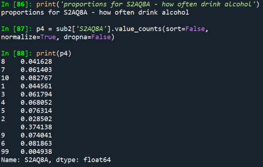
sub1=Data[(Data['AGE']>=21)] sub2=sub1.copy() print('counts for S2AQ8A - how often drink alcohol') c4 = sub2['S2AQ8A'].value_counts(sort=False, dropna=False) print(c4) print('proportions for S2AQ8A - how often drink alcohol') p4 = sub2['S2AQ8A'].value_counts(sort=False, normalize=True, dropna=False) print(p4) print('counts for S2AQ8B - number of drinks') c5 = sub2['S2AQ8B'].value_counts(sort=False, dropna=False) print(c5) print('proportions for S2AQ8B - number of drinks') p5 = sub2['S2AQ8B'].value_counts(sort=False, normalize=True, dropna=False) print(p5) print('counts for S2AQ10 - how often drink enough to feel intox') c6 = sub2['S2AQ10'].value_counts(sort=False, dropna=False) print(c6) 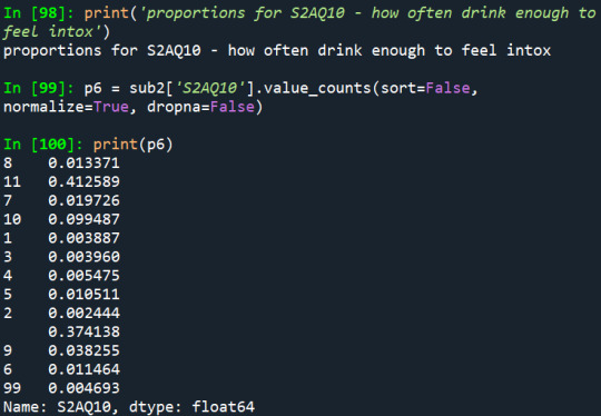print('proportions for S2AQ10 - how often drink enough to feel intox') p6 = sub2['S2AQ10'].value_counts(sort=False, normalize=True, dropna=False) print(p6) print('counts for S2BQ1A1 - feel that usual no. 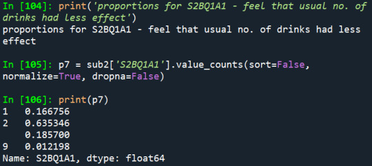of drinks had less effect') c7 = sub2['S2BQ1A1'].value_counts(sort=False, dropna=False) print(c7) print('proportions for S2BQ1A1 - feel that usual no. of drinks had less effect') p7 = sub2['S2BQ1A1'].value_counts(sort=False, normalize=True, dropna=False) print(p7) print('counts for S2BQ1A9B - shake when effects were wearing off') c8 = sub2['S2BQ1A9B'].value_counts(sort=False, dropna=False) print(c8) print('proportions for S2BQ1A9B - shake when effects were wearing off') p8 = sub2['S2BQ1A9B'].value_counts(sort=False, normalize=True, dropna=False) print(p8)

##############################

Here are 3 of the variables I’ve chosen to work with: how often they drink enough to feel intoxicated; and if they have ever felt that the usual amout of alcohol they drink had less effect

1) How often the person drinks alcohol:

2) How often they drink enough to feel intoxicated:

3) Have they ever felt that the usual amount of alcohol they drink had less effect:  

According to the distribution of the first variable, it is noticeable that the two greater proportions are of people who drink 2-3 times a month (8,1%) and people who drink 1-2 times per year (8,2%), considering the last 12 months.

Another thing that can be noted is that nearly 2% (807 people over 21 years old) had drunk enough to feel intoxicated once a month during the last 12 months, which is a frequency that is relatively common among young people, such as college students. 

And according to the third variable, 16,6% of the sample reported having already felt that the usual amount of alcohol had less effect than before, which is an alarm sign to alcohol dependence. 

Also, in the first two variables, it really draws a lot of attention the fact that the missing data represents most of the proportion of the variables.

#python #biostatistics #statistical analysis #medicine #alcohol #alcohol dependence

[oggistat]

First Assignment

To the first assignment of Wesleyan University’s Data Management and Visualization, I’ve chosen NESARC as the dataset of my project, in order to study specific topics about alcoholism. I’ve decided to study the association between alcohol consumption and alcohol dependence. While reading NESARC’s Codebook, I’ve printed some variables of interest in the sections about the topics I’ve chosen – consumption (2A) and dependence (2B). My primary hypothesis is that the more a person drinks alcohol, the more they are susceptible to becoming addicted to alcohol.

For better understanding the theme, I did a brief review of the recent literature there is about this subject, using the terms “alcohol consumption” and “alcohol dependence” in PubMed, also applying the filter “last 5 years” and, later, “Systematic Review”. That search returned 3 interesting and recent articles.

The first of them was conducted with young students at a municipality in Italy, reporting high prevalence of early initiation of alcohol use, which is, according to WHO (in the “Global Status Report on Alcohol and Health 2014”), associated with increased risk for alcohol dependence and abuse, especially because of the greater period of time the individual uses alcohol by early initiating (1). The second study is a review about the epidemiology of alcohol use in the US, presenting information from NESARC and other studies, and also emphasizes the strong association between alcohol use (duration and quantity) and the incidence of alcohol use disorder (AUD) (2). The third study is a meta-analysis about alcohol use and mortality, reporting a very interesting finding: there was no difference between lifetime abstainers and low-volume alcohol consumers, but the mortality was higher in high-volume alcohol consumers. However, the authors strongly reaffirm the high probability of bias in the studies analyzed, because of confounding factors and misclassifying the alcohol use of patients, emphasizing that we need to be skeptical about wether “healthy quantities” of alcohol is a real thing (3).

 1)      https://www.ncbi.nlm.nih.gov/pmc/articles/PMC6069403/pdf/jpmh-2018-02-e167.pdf

2)      https://www.ncbi.nlm.nih.gov/pmc/articles/PMC4872616/pdf/arcr-38-1-7.pdf

3)      https://www.ncbi.nlm.nih.gov/pmc/articles/PMC4803651/pdf/jsad.2016.77.185.pdf

#AlcoholAbuse AlcoholUse LiteratureReview ProjectBasedLearning