#isnulated overalls

[ares857]

internet finds

If you want this project to continue, you can use the Paypal donation button on the web page of the blog. Any donation is welcome.

#overalls #snowbib #snow bib #snow bibs #snowbibs #skibib #ski bib #skibibs #ski bibs #cool #cool look #snow #winter #snoveralls #hoodie #beanie #mask #isnulated overalls #boys and girls

[atillathebunny]

Frequency distributions

I decided to try to do my project in both SAS and Python because I want to learn as much as possible in terms of the tools I can use to analyze data.

SAS 

Because I am not in the US, I was unable to join the SAS course in the US, but I had no problem writing a program from the tutorials and could access the necessary data. So YAY first problem solved.

Here is my program to create 3 frequency tables:

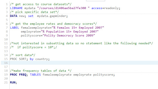
Now the tricky part here is that two of my data categories are continuous, so that makes these tables a bit long.  So I have made the decision not to post the whole table, but just the beginning as otherwise this post would be very very long.  On the continious data my descriptions will be based on the cumulative percent column as most of the frequencies are just 1 or 2 data points and therefore meaningless.

So my first table is female empoyment rate.

This table had 35 missing values and is quite long having values between 11.3% to 83.3%.  A quarter of the employment rates were 38.7% and below, half were 47.5% and below and three quarters were 56% and below.  This shows that woman are not a strong presence in many workforces, expecially when compared to the % of all people employed (scroll down to continue)

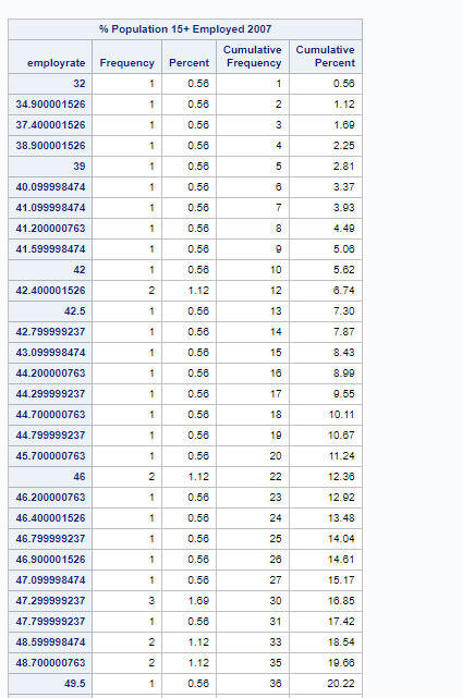
So my second table is overall empoyment rate.

This table also had 35 missing values and is quite long having values between 32% to 83.2%.  A quarter of the employment rates were 51.2% and below, half were 58.6% and below and three quarters were 65.1% and below.  As stated before, as the overall workforce figures are generally higher than the female workforce figures, men are employed at a higher rate then women across the world.  (scroll down to continue)

My last table is democracy score.

As this table is categorical, the whole table is included.

This table also had 52 missing values.  All scores are from -10, the least democratic to 10, the mot democratic. Only 28.57% of countries have negative scores.  And most of the denocratic countries have higher scores.  50% of the scores are 6 and above.  This means that in general we live in a highly democratic world overall, despite some countries still facing autocratic rule.

python

I found python was a bit tricker in terms of its output not being as pretty.  So at least in terms of frequency tables I have a preference for SAS over python in terms of the results being in a user friendly form.

Additionally, I used the internet to determine what some of my errors were in my first coding.  For example I had to add “errors = coerce" when trying to convert my data to numeric.  

I found that for my data, it was better to use the group by method as it sorted my data by value.  However as a result it did not tell me how many NA’s there were.  After a bit of research I found that by combining “isnull()” with “sum()” I could count my null values.

Here is my final code:

# -*- coding: utf-8 -*- """ Script to load in gapminder data and get frequency values and percentages of female employment rates, population employment rates, and democracy scores """ # load libraries import pandas as pd # it appears numpy is not used here import numpy as np

# load data data = pd.read_csv(    'D:/Users/jesnr/Dropbox/coursera/data management and visualization/gapminder data.csv', low_memory=(False))

# toprevent runtime errors #pd.set_option('display.float_format', lambda x: '%f'%x)

# change data to numeric data['femaleemployrate'] = pd.to_numeric(    data['femaleemployrate'], errors='coerce') data['employrate'] = pd.to_numeric(data['employrate'], errors='coerce') data['polityscore'] = pd.to_numeric(data['polityscore'], errors='coerce')

# print the frequency values and percentages feemprateval = data.groupby('femaleemployrate').size() feemprateper = data.groupby('femaleemployrate').size()*100/(len(data)-data['femaleemployrate'].isnull().sum())

print("count of % females 15 and over employed 2007") print(feemprateval) print("percentages of % females 15 and over employed 2007") print(feemprateper) print("missing values in female employment rate data") print(data['femaleemployrate'].isnull().sum()) print()

emprateval = data.groupby('employrate').size()emprateper = data.groupby('employrate').size()*100/(len(data)-data['employrate'].isnull().sum())

print("count of % population  15 and over employed 2007") print(emprateval) print("percentages of % population 15 and over employed 2007") print(emprateper) print("missing values in female employment rate data") print(data['employrate'].isnull().sum()) print()

dempval = data.groupby('polityscore').size() demper = data.groupby('polityscore').size()*100/(len(data)-data['polityscore'].isnull().sum())

print("count of % polity democracy score 2009") print(dempval) print("percentages of % polity democracy score 2009") print(demper) print("missing values in female employment rate data") print(data['polityscore'].isnull().sum()) print()

Please note that my analysis is identical to above because the numbers are all the same, as they should be.  If they hadn’t been it would have indicated an error on my part

Now the tricky part here is that two of my data categories are continuous, so that makes these tables a bit long.  Python agreed and truncated the output.  So I have posted exactly what python outputted.On the continious data my descriptions will be based on the cumulative frequencies which i added up manually as most of the frequencies are just 1 or 2 data points and we were not taught how to do the cummulative frequencies yet.

So my first table is female empoyment rate.

This table had 35 missing values and is quite long having values between 11.3% to 83.3%.  A quarter of the employment rates were 38.7% and below, half were 47.5% and below and three quarters were 56% and below.  This shows that woman are not a strong presence in many workforces, expecially when compared to the % of all people employed (scroll down to continue)

count of % females 15 and over employed 2007 femaleemployrate 11.300000    1 12.400000    1 13.000000    1 16.700001    1 17.700001    1            .. 79.199997    1 80.000000    1 80.500000    1 82.199997    1 83.300003    1 Length: 153, dtype: int64 percentages of % females 15 and over employed 2007 femaleemployrate

11.300000    0.561798 12.400000    0.561798 13.000000    0.561798 16.700001    0.561798 17.700001    0.56179879.199997    0.561798 80.000000    0.561798 80.500000    0.561798 82.199997    0.561798 83.300003    0.561798

Length: 153, dtype: float64

missing values in female employment rate data 35

So my second table is overall empoyment rate.

This table also had 35 missing values and is quite long having values between 32% to 83.2%.  A quarter of the employment rates were 51.2% and below, half were 58.6% and below and three quarters were 65.1% and below.  As stated before, as the overall workforce figures are generally higher than the female workforce figures, men are employed at a higher rate then women across the world.  (scroll down to continue)

count of % population  15 and over employed 2007 employrate 32.000000    1 34.900002    1 37.400002    1 38.900002    1 39.000000    1            .. 80.699997    1 81.300003    1 81.500000    1 83.000000    1 83.199997    2 Length: 139, dtype: int64 percentages of % population 15 and over employed 2007 employrate 332.000000    0.561798 34.900002    0.561798 37.400002    0.561798 38.900002    0.561798 39.000000    0.56179880.699997    0.561798 81.300003    0.561798 81.500000    0.561798 83.000000    0.561798 83.199997    1.123596 Length: 139, dtype: float64 missing values in female employment rate data 35

My last table is democracy score.

As this table is categorical, the whole table is included.

This table also had 52 missing values.  All scores are from -10, the least democratic to 10, the mot democratic. Only 28.57% of countries have negative scores.  And most of the denocratic countries have higher scores.  50% of the scores are 6 and above.  This means that in general we live in a highly democratic world overall, despite some countries still facing autocratic rule.

count of % polity democracy score 2009 polityscore -10.0     2 -9.0      4 -8.0      2 -7.0     12 -6.0      3 -5.0      2 -4.0      6 -3.0      6 -2.0      5 -1.0      4 0.0      6 1.0      3 2.0      3 3.0      2 4.0      4 5.0      7 6.0     10 7.0     13 8.0     19 9.0     15 10.0    33 dtype: int64 percentages of % polity democracy score 2009 polityscore -10.0     1.242236 -9.0      2.484472 -8.0      1.242236 -7.0      7.453416 -6.0      1.863354 -5.0      1.242236 -4.0      3.726708 -3.0      3.726708 -2.0      3.105590 -1.0      2.484472 0.0      3.726708 1.0      1.863354 2.0      1.863354 3.0      1.242236 4.0      2.484472 5.0      4.347826 6.0      6.211180 7.0      8.074534 8.0     11.801242 9.0      9.316770 10.0    20.496894 dtype: float64 missing values in female employment rate data 5232.000000    0.561798 34.900002    0.561798 37.400002    0.561798 38.900002    0.561798 39.000000    0.56179880.699997    0.561798 81.300003    0.561798 81.500000    0.561798 83.000000    0.561798 83.199997    1.123596

#data science #coursera

[jtallhag-blog]

Coursera: Data Management and Visualization - Assignment 4

This blog post is written as part of assignment 4 in the Coursera course Data Management and Visualization. Please note that parts of the code has been carried over from previous assignments but is included here as well for completeness.

I have chosen to use the Gapminder dataset to answer the question of whether there is any evidence to suggest a connection between internet use rate and HIV rate. The background for this question is that I believe that there could be a causal mechanism where increased access to the internet makes information about HIV prevention more available which could make increased internet usage lead to decreased HIV prevalence. There are several possible confounding factors, one is that internet usage correlates with income which also correlates with HIV rate. Hence any connection between internet use rate and HIV rate could also be due to an underlying correlation between each of these and income. While there are other similar possibilities only income has been examined here and for this reason the incomeperperson column from the dataset has also been included in the following, besides the internetuserate and hivrate columns.

The following code was used for loading, managing and plotting the data:

import pandas as pd import numpy as np import seaborn import matplotlib.pyplot as plt

# Set the path where datasets are stored (relative path used) and select which # set to use, concatenate a text string with the full (i.e. composed of path and # filename) name. inputFilePath = '../dataSets/' inputFileName = '_7548339a20b4e1d06571333baf47b8df_gapminder.csv' inputFile = inputFilePath + inputFileName

# Load the chosen data set into a Pandas DataFrame (df for dataframe) df = pd.read_csv(inputFile)

# Set the country column as index df = df.set_index('country')

# Data management: # The data is imported as text strings but is numeric in nature, in addition # of the text strings are empty (consisting of a single space character) which # stops us from converting to a numeric format. Therefore we replace the empty # strings with NaN values before converting to a numeric type. In this case all # the columns should be treated the same way so it's convenient to use a for-in # statement. for col in list(df.columns):    df[col] = df[col].replace(' ',np.nan).astype('float64')

# I'm primarily interested in the columns which describe internet use rate and # HIV rate, since both of these can be expected to be related to overall wealth # I want to keep track of this variable as well. Hence I construct frequency # tables for these three variables. Because the variables are continuous most # values would have a single occurence if this is done directly, hence bins=5 # is set to get an output that is more readable. Setting this makes Pandas # ignore dropna=False so the number of missing values is calculated and printed # separately, to reduce the amount of typing needed a list of the interesting # columns is used together with a for-in statement.     columnsOfInterest = ['internetuserate','hivrate','incomeperperson'] for col in columnsOfInterest:    print("Column: {}".format(col))    print("Missing values: {}".format(df.loc[df[col].isnull()].shape[0]))    print("Value frequency per bracket:")    print(df[col].value_counts(bins=5,sort=False))    print()

# Plot the distribtuion of the internetuserate column internetuserate_distplot = plt.figure() seaborn.distplot(df['internetuserate'].dropna(),kde=False) plt.xlabel('Internet use rate') plt.ylabel('Frequency') plt.title('2010 Internet users per 100 people\n(data from World Bank)')

# Plot the distribtuion of the hivrate column hivrate_distplot = plt.figure() seaborn.distplot(df['hivrate'].dropna(),kde=False) plt.xlabel('HIV rate') plt.ylabel('Frequency') plt.title('2009 estimated HIV prevalence in percent, ages 15-49\n(data from UNAIDS online database)')

# Plot the distribution of the incomeperperson column incomeperperson_distplot = plt.figure() seaborn.distplot(df['incomeperperson'].dropna(),kde=False) plt.xlabel('Income per person') plt.ylabel('Frequency') plt.title('2010 GDP per capita in constant 2000 USD\n(data from World Bank Development Indicators)')

# Plot HIV rate vs. internet use rate, include a fit line to get an indication # of how these correlate     plt.figure() seaborn.regplot(x='internetuserate',y='hivrate',fit_reg=True,data=df) plt.xlabel('Internet use rate (internet users per 100 people)') plt.ylabel('HIV rate (% of population age 15-49 with HIV)') plt.title('HIV rate as function of internet use rate')

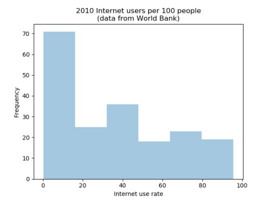
A distribution plot of the internet use rate shows that it has two modi, one at low values centered around 10% (10 internet users per 100 people) and one around 40%. The distribution between other brackets is fairly even.

The HIV rate has a more extreme distribution with most countries clustered around a very pronounced mode centered at a rate of roughly 0.5%, and most remaining ones following an approximately normal distribution (but with the lower half cut off since negative values are not possible) around this value with a slight tendency towards a mode at roughly 3%. However the tail of this distribution shows a number of outlying cases with the highest falling above 25%.

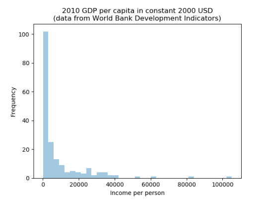
GDP per capita also has a strong concentration around a mode centered at the lowest values with a tendency towards a further mode at around $25 000/year. The tail shows a number of outliers which on closer examination turn out to small tax havens like Monaco or Liechtenstein whose GDPs are dominated by the financial services sector, hence these cases are extreme in the sense of how their economies are structured rather than in real-economy performance.

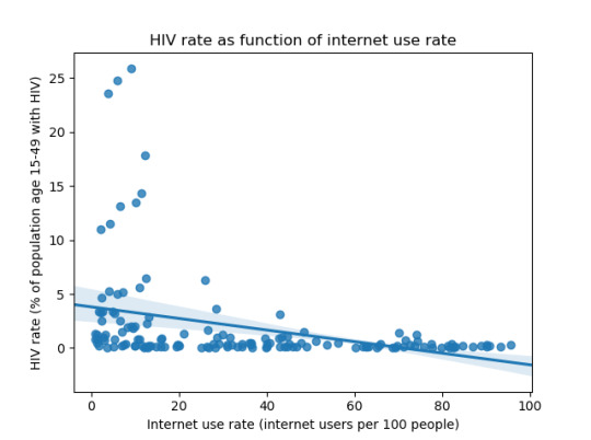
Finally I have plotted HIV rate vs. internet use rate to examine the connection between these with internet use rate as explanatory variable and HIV rate as the dependent one. This shows a clear correlation between these variables, a trend line has been included to give an idea about the strength of the correlation. The correlation can be calculated using the myDataFrame.corr() function (this returns a DataFrame containing the correlations between all columns in myDataFrame) which gives a correlation of -0.34 between hivrate and internetuserate. There is also a correlation of -0.20 between hivrate and incomeperperson so it seems likely that some of the hivrate-internetuserate correlation might be due to an underlying correlation between wealth and HIV rate. However this correlation is considerably smaller than that between internet use rate and HIV rate so the proposed causal mechanism between internet use rate and HIV rate still seems plausible. It should be noted that much of the hivrate-internetuserate correlation comes from a small number of outlier cases with unusually high HIV rates. These are typically located in subsaharan Africa and if one calculates the correlation only for countries in this region then a small positive correlation of 0.01 is obtained between HIV rate and internet use rate along with a larger positive correlation of 0.25 between income per person and HIV rate. Further examination of specific countries show that in this region countries with a high HIV rate often have comparably high income levels, for instance Botswana has the highest HIV rate of 24.8% and the third highest level of income in the group. A possible cause of this somewhat counterintuitive connection is that richer countries have better access to HIV medication and thus their HIV rate may decrease more slowly compared to poorer countries where much of the decrease may be due to those afflicted dying from lack of appropriate medical care.

[ares857]

internet finds

#overalls #snowsuit #snow suit #beanie #goggles #boots #skisuit #ski suit #cool #cool look #hot #hot guy #snow #winter #snowboard #snoveralls #isnulated overalls #jumpsuit #coveralls

[ares857]

internet find

If you want this project to continue, you can use the Paypal donation button on the web page of the blog. Any donation is welcome.

#overalls #dungarees #jacket #insulated #isnulated overalls #zip #zip front #zip front overalls #rolled up #rolled up overalls #cool #cool look #hot #hot guy #cute #cute guy #mansbestfriend #dog #mask #turtleneck #black overalls

[ares857]

internet finds

If you want this project to continue you can use the Paypal donation button on the web page of the blog. Any donation is welcome.

#overalls #coveralls #jumpsuit #cute #cute guy #hot #hot guy #beard #snowsuit #snoveralls #snow suit #cool #cool look #isnulated overalls #sneakers #snow coveralls #winter coveralls #winter overalls #skisuit #ski suit

[ares857]

internet finds

If you want this project to continue you can use the Paypal donation button on the web page of the blog. Any donation is welcome.

#overalls #dungarees #snowbibs #snow bibs #skibibs #ski bibs #goggles #beard #cute #cute guy #beanie #cool #cool look #hot #hot guy #insulated #isnulated overalls #snow overalls #snoveralls #snowboard #friends #snow #winter #hoodie #cuet guy

[jtallhag-blog]

Coursera: Data Management and Visualization - Assignment 2

This blog post is written as part of assignment 2 in the Coursera course Data Management and Visualization.

The following code was used for loading the Gapminder dataset and printing frequency tables for the columns internetuserate, hivrate and incomeperperson. Since all these variables are continuous binning was used to produce sensible frequency tables.

import pandas as pd import numpy as np

# Set the path where datasets are stored (relative path used) and select which # set to use, concatenate a text string with the full (i.e. composed of path and # filename) name. inputFilePath = '../dataSets/' inputFileName = '_7548339a20b4e1d06571333baf47b8df_gapminder.csv' inputFile = inputFilePath + inputFileName

# Load the chosen data set into a Pandas DataFrame (df for dataframe) df = pd.read_csv(inputFile)

# Set the country column as index df = df.set_index('country')

# Data management: # The data is imported as text strings but is numeric in nature, in addition # of the text strings are empty (consisting of a single space character) which # stops us from converting to a numeric format. Therefore we replace the empty # strings with NaN values before converting to a numeric type. In this case all # the columns should be treated the same way so it's convenient to use a for-in # statement. for col in list(df.columns):    df[col] = df[col].replace(' ',np.nan).astype('float64')

# I'm primarily interested in the columns which describe internet use rate and # HIV rate, since both of these can be expected to be related to overall wealth # I want to keep track of this variable as well. Hence I construct frequency # tables for these three variables. Because the variables are continuous most # values would have a single occurence if this is done directly, hence bins=5 # is set to get an output that is more readable. Setting this makes Pandas # ignore dropna=False so the number of missing values is calculated and printed # separately, to reduce the amount of typing needed a list of the interesting # columns is used together with a for-in statement.     columnsOfInterest = ['internetuserate','hivrate','incomeperperson'] for col in columnsOfInterest:    print("Column: {}".format(col))    print("Missing values: {}".format(df.loc[df[col].isnull()].shape[0]))    print("Value frequency per bracket:")    print(df[col].value_counts(bins=5,sort=False))    print()

When run the code produces the following output:

Column: internetuserate Missing values: 21 Value frequency per bracket: (0.114, 19.296]     73 (19.296, 38.381]    35 (38.381, 57.467]    37 (57.467, 76.553]    24 (76.553, 95.638]    23 Name: internetuserate, dtype: int64

Column: hivrate Missing values: 66 Value frequency per bracket: (0.0332, 5.228]     134 (5.228, 10.396]       4 (10.396, 15.564]      5 (15.564, 20.732]      1 (20.732, 25.9]        3 Name: hivrate, dtype: int64

Column: incomeperperson Missing values: 23 Value frequency per bracket: (-1.269, 21112.508]        162 (21112.508, 42121.241]      24 (42121.241, 63129.973]       2 (63129.973, 84138.705]       1 (84138.705, 105147.438]      1 Name: incomeperperson, dtype: int64

All columns have some missing values, the HIV rate one stands out with a very large proportion (roughly a third of the values are missing). The distribution of internet use rate is fairly even but does have skew towards the lowest bracket where between 0.1% and 19.3% of the population have access to the internet. Both HIV rate and income per person are heavily skewed towards the lowest bracket. In the case of incomeperperson it is also interesting to note that the two top brackets contain only one country each. These two outliers are Liechtenstein and Monaco (top bracket) which are both small tax havens where a large share of the GDP (which the incomeperperson column is based on) comes from the banking sector rather than the real economy and is therefore somewhat fictional (see https://en.wikipedia.org/wiki/FISIM for a brief summary about how GDP contributions from the financial sector is calculated), some other top countries like Luxembourg and Bermuda share similar traits. Hence there would be a strong argument for removing these from any analysis as the way their economies are structured are very untypical and including them is likely to obscur rather than enlighten. It is also interesting to note a pattern in the values for HIV rate where the countries with high rates are typically located in sub-saharan Africa. It seems like a reasonable assumptions that these countries may share similar circumstances, for instance many of them have only recently gone through decolonialization after a long period of foreign rule and their political situations are often still heavily affected by this recent history of anti-colonial resistance. Hence there may be an argument for analysing this group separately and possibly comparing them with e.g. south-east Asian countries which share a recent history of colonial rule and independence struggle.

[jtallhag-blog]

Coursera: Data Management and Visualization - Assignment 3

This blog post is written as part of assignment 3 in the Coursera course Data Management and Visualization. Please note that it mostly identical to the post made for assignment 2 since the assignment instructions are very similar and the grading rubrics are identical. The instructions seem differ mainly in assignment 3 calling for data managment to be done which assignment 2 does not even though the rubric includes data management as one of the grading criteria. Since I had included data management decisions (these are explained in the code comments) already in assignment 2 I cannot see any changes which would have been reasonable to make for assignment 3 so I’ve decided to reuse the same code and therefore the same explanatory text as well. I have posted a question in the course forums about what the differences between the two assignments should be but haven’t gotten any reply yet, I may update either or both assignments if I get one.

The following code was used for loading the Gapminder dataset and printing frequency tables for the columns internetuserate, hivrate and incomeperperson. Since all these variables are continuous binning was used to produce sensible frequency tables.

import pandas as pd import numpy as np

# Set the path where datasets are stored (relative path used) and select which # set to use, concatenate a text string with the full (i.e. composed of path and # filename) name. inputFilePath = '../dataSets/' inputFileName = '_7548339a20b4e1d06571333baf47b8df_gapminder.csv' inputFile = inputFilePath + inputFileName

# Load the chosen data set into a Pandas DataFrame (df for dataframe) df = pd.read_csv(inputFile)

# Set the country column as index df = df.set_index('country')

# Data management: # The data is imported as text strings but is numeric in nature, in addition # of the text strings are empty (consisting of a single space character) which # stops us from converting to a numeric format. Therefore we replace the empty # strings with NaN values before converting to a numeric type. In this case all # the columns should be treated the same way so it's convenient to use a for-in # statement. for col in list(df.columns):   df[col] = df[col].replace(' ',np.nan).astype('float64')

# I'm primarily interested in the columns which describe internet use rate and # HIV rate, since both of these can be expected to be related to overall wealth # I want to keep track of this variable as well. Hence I construct frequency # tables for these three variables. Because the variables are continuous most # values would have a single occurence if this is done directly, hence bins=5 # is set to get an output that is more readable. Setting this makes Pandas # ignore dropna=False so the number of missing values is calculated and printed # separately, to reduce the amount of typing needed a list of the interesting # columns is used together with a for-in statement.     columnsOfInterest = ['internetuserate','hivrate','incomeperperson'] for col in columnsOfInterest:   print("Column: {}".format(col))   print("Missing values: {}".format(df.loc[df[col].isnull()].shape[0]))   print("Value frequency per bracket:")   print(df[col].value_counts(bins=5,sort=False))   print()

When run the code produces the following output:

Column: internetuserate Missing values: 21 Value frequency per bracket: (0.114, 19.296]     73 (19.296, 38.381]    35 (38.381, 57.467]    37 (57.467, 76.553]    24 (76.553, 95.638]    23 Name: internetuserate, dtype: int64

Column: hivrate Missing values: 66 Value frequency per bracket: (0.0332, 5.228]     134 (5.228, 10.396]       4 (10.396, 15.564]      5 (15.564, 20.732]      1 (20.732, 25.9]        3 Name: hivrate, dtype: int64

Column: incomeperperson Missing values: 23 Value frequency per bracket: (-1.269, 21112.508]        162 (21112.508, 42121.241]      24 (42121.241, 63129.973]       2 (63129.973, 84138.705]       1 (84138.705, 105147.438]      1 Name: incomeperperson, dtype: int64

All columns have some missing values, the HIV rate one stands out with a very large proportion (roughly a third of the values are missing). The distribution of internet use rate is fairly even but does have skew towards the lowest bracket where between 0.1% and 19.3% of the population have access to the internet. Both HIV rate and income per person are heavily skewed towards the lowest bracket. In the case of incomeperperson it is also interesting to note that the two top brackets contain only one country each. These two outliers are Liechtenstein and Monaco (top bracket) which are both small tax havens where a large share of the GDP (which the incomeperperson column is based on) comes from the banking sector rather than the real economy and is therefore somewhat fictional (see https://en.wikipedia.org/wiki/FISIM for a brief summary about how GDP contributions from the financial sector is calculated), some other top countries like Luxembourg and Bermuda share similar traits. Hence there would be a strong argument for removing these from any analysis as the way their economies are structured are very untypical and including them is likely to obscur rather than enlighten. It is also interesting to note a pattern in the values for HIV rate where the countries with high rates are typically located in sub-saharan Africa. It seems like a reasonable assumptions that these countries may share similar circumstances, for instance many of them have only recently gone through decolonialization after a long period of foreign rule and their political situations are often still heavily affected by this recent history of anti-colonial resistance. Hence there may be an argument for analysing this group separately and possibly comparing them with e.g. south-east Asian countries which share a recent history of colonial rule and independence struggle.