#x1 locs | Explore Tumblr Posts and Blogs

ghoulete · 1 year

Text

➷ 🦷 ⌅ ◌ ⁷⁷⁷

289 notes · View notes

hcneyrq · 2 years

Text

ׄ ִ ∗ you've been waiting to unwrap me 🦤 𓂂 ﾟ∗

304 notes · View notes

90ekz · 5 months

Text

JJK MENS’ FAVORITE SEX THINGS x1

- feat… satoru, toji, todo, higuruma.

- cont… nsfw, very poor dirty talk (someone teach me how to write ts PLEASE), black!fem!reader, typical dom/sub dynamics, sassy men, established relationships, ts nastyyyyy.

- an… ik this is a kinda random bunch, but i wanted to include some underrated men in here !! pt 2 will be up soon with the favs, don’t worry ;)

GOJO SATORU & FINGERING

this man right here… menace to society.

something about massaging your swollen clit with his thumb while he abuses your g-spot with his three fingers of choice is his favorite thing in the world !!!

using his hands during sex in general is a go-to, he knows exactly what it does to you too mmhm.

something about the way you seem to fall apart so much quicker when he uses his hands, watching so intently as he uses his other to press down on your stomach cs it overstims you :(( hes mean i fear

“mm, yeah? that’s that spot right there baby?”

and GOD FORBID you start complaining about how it’s too much, his lil dumbass is smirking and massaging even deeper while tears start to flow down your warm cheeks. asshole vibes 🙄

“awww you cryin’? such a big girl, i know you can give me one more..”

AOI TODO & TIT-FUCKING

to clarify, he didn’t even know you could do this LMFAO

he’d been eyeing your plush chest all night, the top of your dark areolas peaking above your lounging tank. you being you, you were very aware of this fact, and you indulged him. hugging him from behind, “dropping something down your shirt” and asking him to check for it, all the cliches. that man was blushing bhaddd.

eventually he got so needy and asked you to fuck him like a loser :((

so imagine his surprise when you wet his cock with saliva and begin to massage it between your tits, all the while asking him to tell you how it feels. you pushed your boobs together to tighten around him, not at all missing how his breath stuttered in his chest. that man was starstruck and had to hold back his nut fr :/

“ouuu shit—make that dick cum mama…”

now everytime you wear those low cut shirts around your apartment, hes pulling himself out half mast and slapping it on your plush skin, silently demanding.

TOJI FUSHIGURO & BACKSHOTS

do not get me starteddddd.

he adores watching you come back and grind against his dick, meeting him in the middle. the jiggle of your ass is enough to make him drool with a maniacal smile set on his face.

he’s constantly spilling a mix of praise and degradation, how you’re “such a good slut,” and such. he’ll even let you suck on his fingers if he’s gracious.

he’ll yank up any hairstyle you have at the moment and pound into you even deeper. one hand in your hair, another pressing your arch down to his satisfaction. sometimes if he’s feeling sadistic, he’ll won’t move at all and just admire your rhythm against his cock.

“that’s it, there’s my girl… work for that nut.”

as much as you love toji, your hairstylist does not admire him as much as you do. her personal beef has gone on for the entire 2 year length of your relationship that he’s been fuckin’ up lace glue, pulling out braids, unraveling locs, and frizzing up twists, and she has to be the one to fix ‘em… poor girl :/

HIRUMI HIGURUMA & FACE-SITTING

#1 munch award goes to:

you were being very wary about this, considering it isn’t exactly the safest thing to put all of your weight on top of someone’s face and neck but… he hates breathing apparently ??

you feel his rare smile against your sopping wet hole, and his nose bumping against your clit as you grind rhythmically. his nails print crescents into your thighs and he keeps you in place, and he thinks he could die happy right here.

your slick is dripping down his chin, and his dick is so, so stiff. it’s uncanny how committed he is to this, almost like it’s a job—a duty—to please you.

it’s only when you pull away to let him breathe (a notion that he already established that he didn’t need to do) is his smile replaced with a slight scowl, and he’s mumbling into your thighs for you to keep going.

“get back up here, ‘m not done.”

like ok you suicidal freak ??

697 notes · View notes

elympios · 1 year

Text

tentative tagging system i'll have to retroactively update (accidentally wrecked my about page trying to link so that's a problem for future me)

[[MORE]]

#x2 = xillia 2

#x1 = xillia 1 (all x1 characters go here even if they're x2 designs)

#zes = zestiria [additional old tags: #tozx, #zn (novel), #mnt (manga)]

#ber = berseria

#rays = rays

#ast = asteria

#ot = other tales/off topic

topics:

#translation = fan translations/commentary

#ceci n'est pas une traduction = my machine translations

#datamining

#official

#adj = adjacent, not specifically tales but i'm making it so

warnings:

#amb = suspiciously ambiguous kresnik posting that is probably meant to be gen but 🤨

#ng = selfcest or incest cw

#partial nudity

relationship tags (platonic stuff included):

#lj = ludger and julius (probably not romantic bc i already sound unhinged enough as it is)

#lv = ludger and victor (probably romantic bc i think it's funny)

#lr = ludger and rowen (only romantic bc i think it's funny)

#el = ludger and elle

#vfe = victor(!ludger) and fractured asteria elle

#ar = alisha and rose (either, im lazy with this one)

#ms = mikleo and sorey (either, im lazy with this one)

removing rowen/ludger from the #ng tag bc rowen/ludger is already exclusively romantic so there's no need to include it and the only other things i ship are. uh... basically all cw-able for one reason.

x2 tags:

#bad end best end = julius ending my dearly beloved

#loneliest end = ludger ending my dearly beloathed

#chosen end = elle ending my. im actually ambiguously ambivalent.

#murder daughter = fractured asteria elle my sweet child

#normal niisan behaviour = striborg julius

#family parallels = ludger & julius and ludger & elle and victor & elle and claudia & ludger and--

#pre-canon = sobbing noises

aus:

#role reversal au = berzestyx2 au. it's a long story.

#loc sorey = asteria inspired zesty-verse au where post-canon sorey becomes the new lord of calamity and epileo isn't okay

#perfect end = everyone lives au (might include victor)

#fae au = canonverse violet-eyed elle lives

#v #kaira might recognise this system 😂

2 notes · View notes

dlbanalysis · 14 days

Text

Linear Regression 2.0 (Dummy Variables)

This is another Linear Regression post (using statsmodels) - but this time I wanted to talk about 'dummy variables'.

The overarching idea:

In the previous blog post at some point I mention about having multiple variables in our linear regression model that may (or may not) give us more explanatory power.

In this example we'll look at using a dummy variable (attendance) along with SAT score to give us a more precise GPA output.

The code:

Apologies in advance, I know this is incredibly messy - but I feel like the concept behind what's happening is more important than how it looks at the moment!

------------------------------------------------------------------------------ import numpy as np import pandas as pd import statsmodels.api as sm import matplotlib.pyplot as plt import seaborn as sns sns.set() raw_data = pd.read_csv('1.03.+Dummies.csv') data = raw_data.copy() data['Attendance'] = data['Attdance'].map({'Yes': 1, 'No': 0}) print(data.describe())

#REGRESSION # Following the regression equation, our dependent variable (y) is the GPA y = data ['GPA'] # Our independent variable (x) is the SAT score x1 = data [['SAT', 'Attendance']] # Add a constant. Esentially, we are adding a new column (equal in lenght to x), which consists only of 1s x = sm.add_constant(x1) # Fit the model, according to the OLS (ordinary least squares) method with a dependent variable y and an idependent x results = sm.OLS(y,x).fit() # Print a nice summary of the regression. results.summary()

plt.scatter(data['SAT'],y) yhat_no = 0.6439 + 0.0014*data['SAT'] yhat_yes = 0.8665 + 0.0014*data['SAT'] fig = plt.plot(data['SAT'],yhat_no, lw=2, c='#a50026') fig = plt.plot(data['SAT'],yhat_yes, lw=2, c='#006837') plt.xlabel('SAT', fontsize = 20) plt.ylabel('GPA', fontsize = 20) plt.scatter(data['SAT'],data['GPA'], c=data['Attendance'],cmap='RdYlGn')

# Define the two regression equations (one with a dummy = 1 [i.e 'Yes'], the other with dummy = 0 [i.e 'no']) yhat_no = 0.6439 + 0.0014*data['SAT'] yhat_yes = 0.8665 + 0.0014*data['SAT']

# Original regression line yhat = 0.0017*data['SAT'] + 0.275

#Plot the two regression lines fig = plt.plot(data['SAT'],yhat_yes, lw=2, c='#006837', label ='Attendance > 75%') fig = plt.plot(data['SAT'],yhat_no, lw=2, c='#a50026', label ='Attendance < 75%') # Plot the original regression line fig = plt.plot(data['SAT'],yhat, lw=3, c='#4C72B0', label ='original regression line') plt.legend(loc='lower right')

plt.xlabel('SAT', fontsize = 20) plt.ylabel('GPA', fontsize = 20) plt.show()

------------------------------------------------------------------------------

When you run the code, this is the graph you will get!

What am I looking at?

This graph is showing us students' SAT scores against their GPA. It is also showing us regression lines of attendance. In green, we have those students who attended more than 75% and in red, those students who had less than 75% attendance. We can clearly see that the students who had an attendance rate of over 75% are expected to achieve a higher GPA.

How was it done?

Obviously you could find that out by looking at the code - but I want to break it down into steps (for my own benefit in the future if nothing else!)

The first noticeable thing that is different from the previous blog post is we have loaded in the dataset into a variable called 'raw_data' (as opposed to 'data). This is because we have some extra work to do before we get started! *Just an aside here that in the 'Attendance' column we have 'Yes' or 'No' entries depending on whether or not the student has attendance rate of more than 75%.

The next two lines of code:

data = raw_data.copy()

data['Attendance'] = data['Attendance'].map({'Yes': 1, 'No': 0})

The first line will make a copy of our 'raw data' variable and call it 'data'. The next line maps all 'Yes' entries in the 'Attendance' column to 1 and all 'No' entries to 0. As below

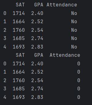
(we only see 5 entries here because both instances [i.e first section is the original and the second one is after the mapping] were printed with the 'data.head()' method).

3. The next thing we need to do is declare our dependent (y) and indedpendent (x1) variables, which are:

y = data ['GPA'] x1 = data [['SAT', 'Attendance']]

4. Once we have this it is the same as before, use statsmodels to create a constant and print some useful statistics!

x = sm.add_constant(x1) results = sm.OLS(y,x).fit() print(results.summary())

A couple of things to note here, the adjusted R-squared value (0.555) is a great improvement from the linear regression we peformed without attendance (0.399) [a note here to say that R-Squared and Adjusted R-Squared will get their own post one day!].

5. So, we can start constructing the equations now. So, our original one was: GPA = 0.275 + 0.0017*SAT

The model including the dummy variable is: GPA = 0.6429 + 0.0014*SAT + 0.2226*Dummy So now, we can split out this dummy variable into two equations (one that has a dummy value of '1' for the attendance greater than 75% and one that has a dummy value of '0' for the attendance less than 75%).

Attended (dummy = 1)

GPA = 0.8665 + 0.0014 * SAT

Did not attend (dummy = 0)

GPA = 0.6439 + 0.0014 * SAT

6. The next line of code is plotting the points in a scatter chart

7. After the points have been plotted we then define our regression lines (as mentioned above):

yhat_no = 0.6439 + 0.0014*data['SAT'] yhat_yes = 0.8665 + 0.0014*data['SAT']

8. Something that I wasn't sure about was one of the arguments in the plt.scatter function. This was the 'cmap='RdYlGn'' parameter. Obviously it is some sort of mapping (Red, Yellow, Green?) but the interesting thing about it was that originally it was 'cmap='RdYlGn_r'' - but I think this reversed the colours or something. Anyway, after I removed the '_r' I was able to display the <75% attendance data points in red which I thought was more intuitive.

9. For reference, perhaps it is a good idea to include our original regression line, this is:

yhat = 0.0017*data['SAT'] + 0.275 10. In the last few lines of code we are plotting the regression lines and giving them titles!

fig = plt.plot(data['SAT'],yhat_yes, lw=2, c='#006837', label ='Attendance > 75%') fig = plt.plot(data['SAT'],yhat_no, lw=2, c='#a50026', label ='Attendance < 75%') # Plot the original regression line fig = plt.plot(data['SAT'],yhat, lw=3, c='#4C72B0', label ='original regression line') plt.legend(loc='lower right')

plt.xlabel('SAT', fontsize = 20) plt.ylabel('GPA', fontsize = 20) plt.show()

So there you have it, that is our linear regression with a dummy variable. I thought that was really interesting. Quite a clever trick to convert categorical data into something numeric like that (but i suppose a binary outcome like 'yes' or 'no' is kind of easy enough I suppose - next time it'd be interesting to see how its done with something like eye colour [blue, green, brown, hazel etc].

0 notes

caqeqimixehi · 2 years

Text

Formulaire demande d'emploi metro

FORMULAIRE DEMANDE D'EMPLOI METRO >> DOWNLOAD LINK vk.cc/c7jKeU

FORMULAIRE DEMANDE D'EMPLOI METRO >> READ ONLINE bit.do/fSmfG

entretien d'embauche metro metro emploi étudiant metro candidature spontanée metro recrutement metro recrutement alternance indeed metroles avantages de travailler chez metro la metro grenoble recrutement

Nouveau : un portail de recrutement pour toutes vos candidatures; Offres d'emploi de Grenoble Alpes Métropole; Candidature spontanée; Offres et demande de Chacun peut vivre un parcours professionnel riche chez METRO France. Venez découvrir nos offres d'emploi. Plus de 300 métiers dédiés à la gastronomie ! J'atteste que les renseignements contenus dans cette demande d'emploi sont conformes à la vérité. Je consens à ce Veuillez remplir le formulaire suivant. *Champ obligatoire. Prénom *. Nom de famille *. Courriel *. Numéro de téléphone *. Choisissez un secteur d'activité Et si on travaillait ensemble ? Découvrez tous nos métiers et nos offres d'emploi sur notre site. Postuler à une offre d'emploi · Envoyer une candidature spontanée · Demander un stage ou une alternance · Suivre ma candidature · Autres questions Transports sur le réseau MÉTRO-BUS-TRAMWAY de l'agglomération toulousaine DEMANDEUR D'EMPLOI (domicilié hors du Périmètre des Transports Urbains).Fill Formulaire Demande D'emploi Metro, Edit online. Sign, fax and printable from PC, iPad, tablet or mobile with pdfFiller ✓ Instantly. Try Now!

https://caqeqimixehi.tumblr.com/post/693661484801261568/expulsion-locative-mode-demploi, https://caqeqimixehi.tumblr.com/post/693661236403027968/notice-lenovo-x1-carbon, https://qojorajoh.tumblr.com/post/693662667295113216/silverlit-drone-manual, https://caqeqimixehi.tumblr.com/post/693664073333768193/fritzwlan-repeater-1750e-mode-demploi, https://qojorajoh.tumblr.com/post/693665332347469824/notice-de-montage-piscine-bestway-power-steel.

0 notes

qojorajoh · 2 years

Text

Silverlit drone manual

bsp; <center>SILVERLIT DRONE MANUAL >> <a href="http://vk.cc/c7jKeU" rel="nofollow" target="_blank">DOWNLOAD LINK</a> vk.cc/c7jKeU   SILVERLIT DRONE MANUAL >> <a href="http://bit.do/fSmfG" rel="nofollow" target="_blank">READ ONLINE</a> bit.do/fSmfG   </center>      problème drone silverlit

silverlit spy racer drone instructions

chargeur drone silverlitnotice drone quadcopter

drone silverlit blacksior

silverlit drone mode d'emploi

silverlit drone spy racer

silverlit drone batterie

Drone GPS DR-POWER HD et son masque FPV. EN - User manual - DR-POWER HD drone · FR - Manuel d'utilisation - Drone DR-POWER HD1- Charger la batterie du drone ou changer les piles de la télécommande. 2- Si cela ce produit, éteindre et rallumer l'appareil en suivant les instructions du

https://caqeqimixehi.tumblr.com/post/693661236403027968/notice-lenovo-x1-carbon, https://caqeqimixehi.tumblr.com/post/693661484801261568/expulsion-locative-mode-demploi, https://caqeqimixehi.tumblr.com/post/693661484801261568/expulsion-locative-mode-demploi, https://caqeqimixehi.tumblr.com/post/693661484801261568/expulsion-locative-mode-demploi, https://caqeqimixehi.tumblr.com/post/693661484801261568/expulsion-locative-mode-demploi.

#&n

1 note · View note

auto-rulate-timisoara · 2 years

Text

BMW X1 Verificare + Livrare GRATUITA, 12 Luni Garantie, RATE FIXE, 2.0 DSL, 177 CP, Euro 5, Pret 9999€

BMW X1 Verificare + Livrare GRATUITA, 12 Luni Garantie, RATE FIXE, 2.0 DSL, 177 CP, Euro 5, Pret 9999€, deosebita, arata si functioneaza foarte bine, fara zgarieturi sau alte defecte, este impecabila din toate punctele de vedere. Masina este recent adusa, arata exact ca in poze. Te invitam sa urmaresti si video de prezentare https://is.gd/OOCSDp SC Danove Interauto SRL este cel mai mare parc auto din vestul tarii cu cele mai multe masini second hand pe stoc. Detinem in permanenta pe stoc o gama diversificata de aproximativ 70 de autoturisme pentru care oferim GARANTIE pe o perioada de 3 LUNI fara limita de KM, indiferent de vechimea autoturismului si fara nici un cost suplimentar din partea cumparatorului. Va oferim posibilitatea de a cumpara un autoturism, cu plata pe loc, cash, card sau printr-un sistem avantajos de rate fixe, indiferent de vechimea autoturismului dorit, cu aprobare in maxim 2 ore. Contractul de leasing se incheie la sediul parcului auto, cu un avans cuprins intre 0% si 30% din valoarea autoturismului. - Puteti figura in baza de date la Biroul de Credit - Puteti avea si alte credite - Sunt acceptate persoanele aflate la pensie - Sunt acceptate veniturile din chirii si diurne - Sunt eligibile pentru finantare si persoanele care lucreaza in strainatate - Leasing pentru Persoane Fizice cu avans intre 0%-30% - Leasing pentru Persoane juridice cu avans intre 0%-30% - ASIGURAM NUMERE ROSII SI FACTURA FISCALA PE LOC Contact: 0784 705 690 0743 051 599 Adresa: Strada Constructorilor 38 Dumbravita, langa Timisoara Anunturi auto second hand https://danoveauto.ro/anunturi-auto/ Detalii finantare https://danoveauto.ro/finantare/ Firma detinatoare de certificat de incredere. Nu facem schimburi. #danoveauto #ratefixe #autosecond

0 notes

lo-eyv · 4 years

Text

⠀⠀⠀♥︎: 𖥻 san & hangyul locs.

⠀⠀⠀𝘀 ₊ 𝗁. 聖。𝗒 ˒ જ

⠀⠀⠀ル﹠ 𝘀. ⋄ 𝗮 ִֶָ さ

⠀⠀⠀ꗃ ⸼ 한. 𝗒 ˒ 𝗌 · 산

⠀⠀⠀like or reblog ㅡ @wonyif on tt

#san bios #san locs #san ateez #ateez bios #ateez locs #hangyul bios #hangyul locs #hangyul x1 #x1 bios #x1 locs #bg bios #bg locs #kpop messy bios #kpop messy #kpop bios #kpop locs

315 notes · View notes

youngh00n · 4 years

Text

/ 은상 瑛 ꘩

e͟u͟n͟ %~ * . ☆%𝐁𝐚𝐛𝐘 !!

e̲ 国 ∞ 曉 ҂ 𝘀.

·•᷄‎ࡇ•᷅ ) eunsang locs!! ☄︎

76 notes · View notes

miyarte · 4 years

Text

wonjin and dongpyo bios.

⠀⠀⠀⠀ ⊹🌷̸ܸ 𝘄𝝾𝗻𝗷𝝸𝗇 ﹍冬 ՙՙ 𝗉𝗒𝗼 𓂅

⠀⠀⠀⠀⠀   ᷼ ﹢ 함 ៸៸ 🌿𓈒 손 ꭑⲓ 𝖼𝝰𝘀𝖺 ｡

⠀⠀⠀⠀⠀⠀⠀𓍢 ⊹ 𝘸𝘰𝘯 ﹏ 🎾̸ 𝗉𝗒𝗼 ゅִ ꜄

⠀⠀⠀⠀⠀⠀ ، O𝟣 ☓ O𝟤 ㅀ. 🧤 𖽑𖽑 웄 ७ִ

⠀⠀⠀⠀⠀⠀⠀⠀⠀⠀⠀ like or reblog

⠀⠀⠀⠀ ⠀ ⠀⠀⠀⠀pcysirius on twt

#kpop bios #messy bios #soft bios #kpop packs #kpop soft bios #kpop messy bios #cravity bios #cravity #x1 bios #x1 locs #x1 #dsp dongpyo #wonjin bios #x1 dongpyo #dongpyo bios

77 notes · View notes

izqne · 4 years

Text

⠀⠀ ♥︎ % minhee locs

민희 ? ★ 애기 ! ~ 🎲

$/✿__민희! 🧩

☆__희?! ~ ♥︎ 🍳

倍/☻﹏미니! ‹3 👋🏻

@yuiseok on twt

#minhee #minhee locs #minhee bios #minhee messy #cravity #cravity locs #cravity bios #cravity messy #x1 #x1 locs #x1 bios #x1 messy #kpop locs #messy locs #kpop bios

83 notes · View notes

ipkjk · 4 years

Text

bts & x1 locs

ㅤㅤ ﹟𝒷𝓍 ᤳ 🥡 ꀬ

ㅤㅤo̲n̲e̲ ٫ 𖠿 𓂃 䮾

ㅤㅤꗃ𓈒 ᤴ 🛴 ৲ .

ㅤㅤ𝚋𝟷 . 🌳 love.

ㅤㅤhome 𓂅 ‹𝟹.

like or reblog if you save.

#bts #x1 #bts locs #x1 locs #kpop locs

45 notes · View notes

aki-meno · 4 years

Text

seungyoun locs

⌗ 𝚠𝚘𝚘𝚍𝚣 𓏸 𓈒 〄

ꗃ 𝙨. ⎙

ৎ୭ 🍿 𝐜𝐡𝐨⁹⁶ ！

like or reblog if you save

#kpop bgs #kpop bios #kpop locs #x1 locs #x1 bios #uniq seungyoun #seungyoun bios #bg locs

40 notes · View notes

dlbanalysis · 20 days

Text

Linear Regression

So in my first proper post i'd like to talk a bit about Linear Regression.

In the Data Science course I am studying, we are given an example dataset (real_estate_price_size.csv) to play that contains one column with house price and another with house size. In one exercise, we were asked to create a simple linear regression using this dataset. Here is the code for it:

------------------------------------------------------------------------------

import numpy as np import pandas as pd import matplotlib.pyplot as plt import statsmodels.api as sm import seaborn seaborn.set() import unicodeit

data = pd.read_csv('real_estate_price_size.csv') #using the data.describe() method gives us nice descriptive statistics! print(data.describe())

#y is the dependent variable y = data['price'] #x is the independent variable x1 = data['size']

#add a constant x = sm.add_constant(x1) #fit the model, according to the OLS (ordinary least squares) method with a dependent variable y and independent x results = sm.OLS(y, x).fit() print(results.summary())

plt.scatter(x1,y) #coefficients obtained from the OLS summary. In this case, the property size has the multiplier of 223.1787 and the intercept of 101900 (the constant) yhat = 223.1787*x1 + 101900 fig = plt.plot(x1, yhat, lw=2, color='red', linestyle='dotted', label='Regression line') plt.xlabel(unicodeit.replace('Size (m^2)'),fontsize = 15) plt.ylabel('Price',fontsize = 15) plt.title('House size and price',fontsize =20,loc='center') plt.savefig('LinearRegression_PropertyPriceSize.png')

plt.show()

------------------------------------------------------------------------------

And here is the scatter graph of the data with a regression line!

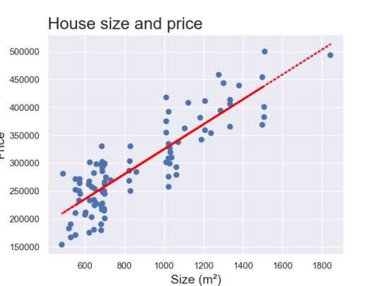
So overall I'm very happy with this. After a bit more playing around i'd like to be able to sort out the y-axis so that the title isn't cut off!

But what does that code actually do?

A couple of things in the code that I'd like to explain:

The first 7 lines (i.e the import numpy etc) are for importing the relevant libraries. By stating something like 'import matplotlib.pyplot as plt' means that each time you want to call on matplotlib.pyplot, you only have to write 'plt'!

The next line of code, "data = pd.read_csv('real_estate_price_size.csv')" is using the pandas library and syntax to load in the real estate data (in comma seperated value [.csv] format).

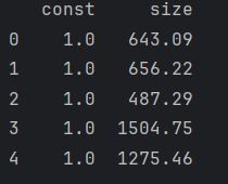
By using "print(data.describe())" we can see a variety of statistics as shown below:

4. After this, the next lines of code are declaring the dependent variable (y) and the independent variable (x1). With regards to the '1' after the 'x' - it's a good habit to get into labelling them in this way (we will see later that we can make our regression more sophisticated [or in some cases not!] by using more than one x term [i.e x1, x2, x3,...,xk]).

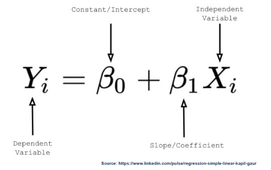
5. The next bit is slightly more complicated - so it's probably worth taking a step back. Remember that a straight line has the equation: y = mx + c, where y = dependent variable, x = independent variable, m = slope and c = intercept (where the line cuts the y-axis). So now imagine that we're trying to fit this line to some data points - we want a constant term c that is non-zero.

A bit of a digression here - but hopefully this will make sense. Imagine that we are trying to predict someones salary based on their years of experience. We collect data on both and we want to fit a line to this data to understand how salary changes with experience.

Even if someone has zero years of experience, they still might have a base salary.

So in regresison analysis, we often include a constant term (or intercept) to account for this baseline value. When you add this constant term to your data, it ensures that the regression model considers this starting salary even if someone has zero years of experience.

This constant term is like the starting point on the salary scale, just like the y-intercept is the starting point on the graph of a straight line.

x = sm.add_constant(x1) will add constants (of 1) as a column next to our 'x1' which in this example is 'size'

So this column of ones corresponds to x0 in the equation

y_hat = b0 * x0 + b1 * x1.

So this means that x0 is always going to be 1, which in turn yields

y_hat = b0 + b1*x1

So now that we've got that cleared up, it's on to the next bit. This is the following section of code:

results = sm.OLS(y, x).fit() print(results.summary())

sm.OLS (Odinary Least Squares) is a method for estimating the parameters in a linear regression model

(y,x) represent the dependent variable we're trying to predict and the indepenedent variable we believe are influencing y.

.fit() this is a function that fits the linear regression model to your data, estimating the coefficients that best describe the relationship between the variables.

results.summary() returns this:

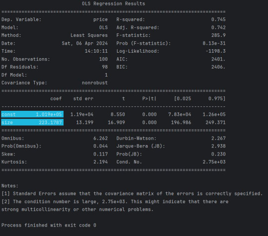
6. The next section is relatively straightforward! This is the bit where we actually plot the data on the graph!

So first of all we have plt.scatter(x1, y) - which is fairly self explanatory!

Next, we declare a new variable yhat. The highlighted sections in the previous image give us the values we need for the equation. So we have 223.1787 (this is our Beta1 that is multiplying x1) and we have 1.019e+05 (which is 101,900) which is our Beta0. I suppose we could have arranged it (so that it is in the same format as the diagram) as yhat = 101900 + 223.1787*x1

So the next bit - I have to be honest - I'm not entirely sure of the arguments and their order, but essentially it looks as if

fig = plt.plot(x1, yhat, lw=2, color='red', linestyle='dotted', label='Regression line')

is determining the attributes of the graph (i.e the variables for the x and y axes, the line width (lw), colour, the style of the line etc).

The next 3 to 4 lines are quite straightforward. Essentially just giving the axes a title, specifying the font size, giving the chart a title and using the plt.savefig() method to save the image!

0 notes

sukvamp · 3 years

Text

## kim yohan layouts 🗯

fav OR reblog if you save

282 notes · View notes