#rgedit
Photo

13 years ago today!
Emma Watson filming the Harry Potter epilogue in London [May 24, 2010]
The scene ended up being reshot months later with a different style for Hermione.
Rupert Grint can also be seen.
All photos at the source
#emma watson#rupert grint#harry potter#emmawatson#rupertgrint#harrypotter#ewedit#emmawedit#ewatsonedit#emmawatsonedit#rgedit#rupertgedit#rgrintedit#rupertgrintedit#hpedit#harrypotteredit
68 notes
·
View notes
Photo


©️ barry gossage
#rebekah gardner#chicago sky#wnba#always smiling <3 even when she's locking your faves the fuck up <3#rgedits#wnbaedits
13 notes
·
View notes
Text
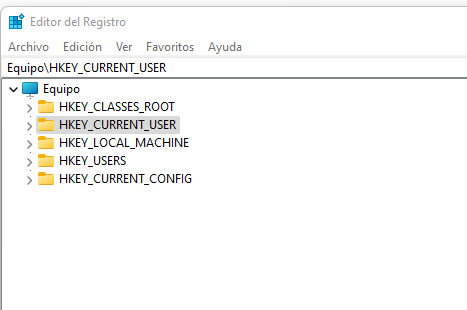
Clave odbc por rgedit
Clave odbc por rgedit
Inicio ->ejecutar ->regedit
HKEY_CURRENT_USER/SOFTWARE/ODBC ->
ABRIR ODBC , DENTRO TENGO LA CLAVE DE UN SISTEMA ADMINISTRATIVO QUE USA MYSQL
todas las que existan por odbc estarán aquí.
View On WordPress
0 notes
Photo


Maurice (1987) | Rupert Graves as Alec Scudder
The girls were damned ugly, which the man wasn't: somehow this made it worse, and he stared at the trio, feeling cruel and respectable; the girls broke away giggling, the man returned the stare furtively and then thought it safer to touch his cap; he had spoilt that little game. But they would meet again when he had passed, and all over the world girls would meet men, to kiss them and be kissed; might it not be better to alter his temperament and toe the line? He would decide after his visit—for against hope he was still hoping for something from Clive. - Maurice E.M. Forster, ch. 34
236 notes
·
View notes
Photo


Daniel Radcliffe , Rupert Grint and Emma Watson (2000).
#rupert grint#emma watson#daniel radcliffe#photoshoot#myedits#celebedit#celebrity#hpcastedit#hpcast#harry potter cast#harry potter#hpedit#ewatsonedit#ewedit#emmawatsonedit#dradcliffeedit#dredit#danielradcliffeedit#rgrintedit#rgedit#rupertgrintedit
157 notes
·
View notes
Photo


Rick Grimes appreciation post [ 2 / ∞ ]
#Rick Grimes#rgedit#The Walking Dead#6x07#my gifs#my edits#my stuff#twdedit#Walking Dead#TWD#AL#Season 6#Church of Rick Grimes#rickgrimesedit#my appreciation post#rickapedit
28 notes
·
View notes
Photo
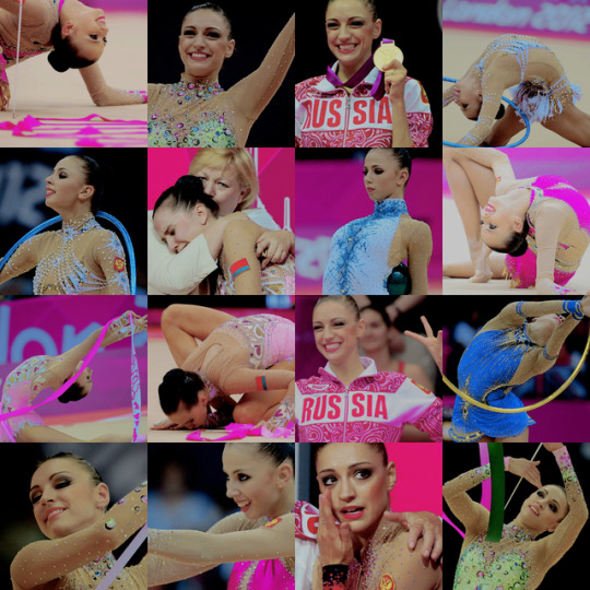
Kanaeva, Dmitrieva, and Charkashyna | London 2012
#evgenia kanaeva#daria dmitrieva#liubov charkashyna#rhythmic gymnastics#rhythmic#rg#rgedit#edit#team russia#russia#belarus#london 2012#olympics
53 notes
·
View notes
Photo


“I've never fancied that footballer lifestyle. I suppose I could live that kind of flash life. People stereotype child actors and kind of expect you to go off the rails a bit, be a bit crazy, but that's not really happened yet.“
#Rupert Grint#rgedit#MyEdit#Quotes#Bad Journalists#Bad articles#Grinters#GrintersFamily#Photoshoot#Actor#Child Actor
38 notes
·
View notes
Photo


It’s something I really relish and it’s something that I haven’t really had the opportunity to do, have a character and really develop it further and really carve out a journey, I think that’s great of the long format of Snatch and not something the film could really touch on. I find it very exciting.
1K notes
·
View notes
Photo


I'm letting life hit me until it gets tired. Then I'll hit back. It's a classic rope-a-dope.
#la la land#lalalandedit#llledit#emma stone#emmastoneedit#esedit#ryan gosling#ryangoslingedit#rgedit#my edit
2K notes
·
View notes
Photo


⚡ABCs Of Harry Potter → R: Ron Weasley
↳ ”Weasley is our King, Weasley is our King, He didn’t let the Quaffle in,
Weasley is our King.
Weasley can save anything, He never leaves a single ring,
That’s why Gryffindors all sing:
Weasley is our King.”
#IVE BEEN WAITING FOR THIS MOMENT#MY TIME TO SHINE#MY SMOL BEAN#MY BABY#MY FATHER SON AND HOLY SPIRIT#okay kate shut up#ABCs of HP#Ron Weasley#harry potter#hpedit#rwedit#rgedit#rupert grint#hpgraphic#mine
323 notes
·
View notes
Photo


#plz#emmerdale#ed#emmerdaleedit#ededit#rhona goskirk#vanessa woodfield#rhona x vanessa#vanessa x rhona#vwedit#rgedit#alcohol /#*#myedits#10.02.2017#otp: i mean me too for you you fool
157 notes
·
View notes
Photo


favourite game day outfits 2022: rebekah gardner
#rebekah gardner#chicago sky#wnba#..........just remembered i have more of these to do fhisfhsw#rgedits#csedits#wnbaedits#game day faves 2022
35 notes
·
View notes
Photo


Me? Heh, heh. I ain't doin' shit.
#The Walking Dead#Rick Grimes#Negan#twdedit#nynas edit#its been a while#i tried!!!! :(#rgedit#nynas gif
26 notes
·
View notes
Text
howdidthe germans decoy it
that
iiiiiiii char ged it
themmmmmm quelledit as takeawayrights
ii iii chargedit
themmm quelledit so to harm anyway theycan
iiiiiiiiicha rgedit
themmmmm reconfirm harmed it sothat it nutloops and thatguy s
an d harmedbiology and repeatedmorecrimes
thatreq uires fuckingup the peoples sense of whats rightandwrong
three four five ten times
thirteentimes
howdidthe germans decoy it
that
iiiiiiii charged it
themmmmmm quelledit as takeawayrights
iiiii chargedit
themmm quelledit so to harm anyway theycan
iiiiiiiiichargedit
themmmmm reconfirm harmed it sothat it nutloops and thatguy s
and harmedbiology and repeatedmorecrimes
thatrequires fuckingup the peoples sense of whats rightandwrong
three four five ten times
thirteentimes
they…
View On WordPress
0 notes
Text
Programming in R
Programming in R
From: http://manuals.bioinformatics.ucr.edu/home/programming-in-r
Author:
Thomas Girke
,
UC Riverside
Contents
1 Introduction
2 R Basics
3 Code Editors for R
4 Integrating R with Vim and Tmux
5 Finding Help
6 Control Structures
7 Functions
8 Useful Utilities
9 Running R Programs
10 Object-Oriented Programming (OOP)
11 Building R Packages
12 Reproducible Research by Integrating R with Latex or Markdown
13 R Programming Exercises
14 Translation of this Page
6.1 Conditional Executions
6.2 Loops
6.1.1 Comparison Operators
6.1.2 Logical Operators
6.1.3 If Statements
6.1.4 Ifelse Statements
6.2.1 For Loop
6.2.2 While Loop
6.2.3 Apply Loop Family
6.2.4 Other Loops
6.2.5 Improving Speed Performance of Loops
6.2.3.1 For Two-Dimensional Data Sets: apply
6.2.3.2 For Ragged Arrays: tapply
6.2.3.3 For Vectors and Lists: lapply and sapply
8.1 Debugging Utilities
8.2 Regular Expressions
8.3 Interpreting Character String as Expression
8.4 Time, Date and Sleep
8.5 Calling External Software with System Command
8.6 Miscellaneous Utilities
10.1 Define S4 Classes
10.2 Assign Generics and Methods
13.1 Exercise Slides
13.2 Sample Scripts
13.2.1 Batch Operations on Many Files
13.2.2 Large-scale Array Analysis
13.2.3 Graphical Procedures: Feature Map Example
13.2.4 Sequence Analysis Utilities
13.2.5 Pattern Matching and Positional Parsing of Sequences
13.2.6 Identify Over-Represented Strings in Sequence Sets
13.2.7 Translate DNA into Protein
13.2.8 Subsetting of Structure Definition Files (SDF)
13.2.9 Managing Latex BibTeX Databases
13.2.10 Loan Payments and Amortization Tables
13.2.11 Course Assignment: GC Content, Reverse & Complement
Introduction
[
Slides
] [
R Code
]
General Overview
One of the main attractions of using the
R (http://cran.at.r-project.org)
environment is the ease with which users can write their own programs and custom functions. The R programming syntax is extremely easy to learn, even for users with no previous programming experience. Once the basic R programming control structures are understood, users can use the R language as a powerful environment to perform complex custom analyses of almost any type of data.
Format of this Manual
In this manual all commands are given in code boxes, where the R code is printed in black, the comment text in blue and the output generated by R in green. All comments/explanations start with the standard comment sign '#' to prevent them from being interpreted by R as commands. This way the content in the code boxes can be pasted with their comment text into the R console to evaluate their utility. Occasionally, several commands are printed on one line and separated by a semicolon ';'. Commands starting with a '$' sign need to be executed from a Unix or Linux shell. Windows users can simply ignore them.
R Basics
The
R & BioConductor
manual provides a general introduction to the usage of the R environment and its basic command syntax.
Code Editors for R
Several excellent code editors are available that provide functionalities like R syntax highlighting, auto code indenting and utilities to send code/functions to the R console.
Basic code editors provided by Rguis
RStudio: GUI-based IDE for R
Vim-R-Tmux: R working environment based on vim and tmux
Emacs (ESS add-on package)
gedit and Rgedit
RKWard
Eclipse
Tinn-R
Notepad++ (NppToR)
Programming in R using Vim or Emacs Programming in R using RStudio
Integrating R with Vim and Tmux
Users interested in integrating R with vim and tmux may want to consult the Vim-R-Tmux configuration page.
Finding Help
Reference list on R programming (selection)
R Programming for Bioinformatics, by Robert Gentleman
Advanced R, by Hadley Wickham
S Programming, by W. N. Venables and B. D. Ripley
Programming with Data, by John M. Chambers
R Help & R Coding Conventions, Henrik Bengtsson, Lund University
Programming in R (Vincent Zoonekynd)
Peter's R Programming Pages, University of Warwick
Rtips, Paul Johnsson, University of Kansas
R for Programmers, Norm Matloff, UC Davis
High-Performance R, Dirk Eddelbuettel tutorial presented at useR-2008
C/C++ level programming for R, Gopi Goswami
Control Structures
Conditional Executions
Comparison Operators
equal: ==
not equal: !=
greater/less than: > <
greater/less than or equal: >= <=
Logical Operators
and: &
or: |
not: !
If StatementsIf statements operate on length-one logical vectors.
Syntax
if(cond1=true) { cmd1 } else { cmd2 }
Example
if(1==0) {
print(1)
} else {
print(2)
}
[1] 2
Table of Contents
Avoid inserting newlines between '} else'.
Ifelse StatementsIfelse statements operate on vectors of variable length.
Syntax
ifelse(test, true_value, false_value)
Example
x <- 1:10 # Creates sample data
ifelse(x<5 | x>8, x, 0)
[1] 1 2 3 4 0 0 0 0 9 10
Table of Contents
Loops
The most commonly used loop structures in R are for, while and apply loops. Less common are repeat loops. The break function is used to break out of loops, and next halts the processing of the current iteration and advances the looping index.
For LoopFor loops are controlled by a looping vector. In every iteration of the loop one value in the looping vector is assigned to a variable that can be used in the statements of the body of the loop. Usually, the number of loop iterations is defined by the number of values stored in the looping vector and they are processed in the same order as they are stored in the looping vector.
Syntax
for(variable in sequence) {
statements
}
Example
mydf <- iris
myve <- NULL # Creates empty storage container
for(i in seq(along=mydf[,1])) {
myve <- c(myve, mean(as.numeric(mydf[i, 1:3]))) # Note: inject approach is much faster than append with 'c'. See below for details.
}
myve
[1] 3.333333 3.100000 3.066667 3.066667 3.333333 3.666667 3.133333 3.300000
[9] 2.900000 3.166667 3.533333 3.266667 3.066667 2.800000 3.666667 3.866667
Table of Contents
Example:
condition*
x <- 1:10
z <- NULL
for(i in seq(along=x)) {
if(x[i] < 5) {
z <- c(z, x[i] - 1)
} else {
z <- c(z, x[i] / x[i])
}
}
z
[1] 0 1 2 3 1 1 1 1 1 1
Table of Contents
Example:
stop on condition and print error message
x <- 1:10
z <- NULL
for(i in seq(along=x)) {
if (x[i]<5) {
z <- c(z,x[i]-1)
} else {
stop("values need to be <5")
}
}
Error: values need to be <5
z
[1] 0 1 2 3
Table of Contents
While LoopSimilar to for loop, but the iterations are controlled by a conditional statement.
Syntax
while(condition) statements
Example
z <- 0
while(z < 5) {
z <- z + 2
print(z)
}
[1] 2
[1] 4
[1] 6
Table of Contents
Apply Loop Family
For T
wo-Dimensional Data Sets: apply
Syntax
apply(X, MARGIN, FUN, ARGs)
X: array, matrix or data.frame; MARGIN: 1 for rows, 2 for columns, c(1,2) for both; FUN: one or more functions; ARGs: possible arguments for function
Example
## Example for applying predefined mean function
apply(iris[,1:3], 1, mean)
[1] 3.333333 3.100000 3.066667 3.066667 3.333333 3.666667 3.133333 3.300000
...
## With custom function
x <- 1:10
test <- function(x) {
# Defines some custom function
if(x < 5) {
x-1
} else {
x / x
}
}
apply(as.matrix(x), 1, test) #
Returns same result as previous for loop*
[1] 0 1 2 3 1 1 1 1 1 1
## Same as above but with a single line of code
apply(as.matrix(x), 1, function(x) { if (x<5) { x-1 } else { x/x } })
[1] 0 1 2 3 1 1 1 1 1 1
Table of Contents
For Ragged Arrays: tapply
Applies a function to array categories of variable lengths (ragged array). Grouping is defined by factor.
Syntax
tapply(vector, factor, FUN)
Example
## Computes mean values of vector agregates defined by factor
tapply(as.vector(iris[,4]), factor(iris[,5]), mean)
setosa versicolor virginica
0.246 1.326 2.026
## The aggregate function provides related utilities
aggregate(iris[,1:4], list(iris$Species), mean)
Group.1 Sepal.Length Sepal.Width Petal.Length Petal.Width
1 setosa 5.006 3.428 1.462 0.246
2 versicolor 5.936 2.770 4.260 1.326
3 virginica 6.588 2.974 5.552 2.026
Table of Contents
For Vectors and Lists: lapply and sapply
Both apply a function to vector or list objects. The function lapply returns a list, while sapply attempts to return the simplest data object, such as vector or matrix instead of list.
Syntax
lapply(X, FUN)
sapply(X, FUN)
Example
## Creates a sample list
mylist <- as.list(iris[1:3,1:3])
mylist
$Sepal.Length
[1] 5.1 4.9 4.7
$Sepal.Width
[1] 3.5 3.0 3.2
$Petal.Length
[1] 1.4 1.4 1.3
## Compute sum of each list component and return result as list
lapply(mylist, sum)
$Sepal.Length
[1] 14.7
$Sepal.Width
[1] 9.7
$Petal.Length
[1] 4.1
##
Compute sum of each list component and return result as vector
sapply(mylist, sum)
Sepal.Length Sepal.Width Petal.Length
14.7 9.7 4.1
Table of Contents
Other Loops
Repeat Loop
Syntax
repeat statement
s
Loop is repeated until a break is specified. This means there needs to be a second statement to test whether or not to break from the loop.
Example
z <- 0
repeat {
z <- z + 1
print(z)
if(z > 100) break()
}
Table of Contents
Improving Speed Performance of LoopsLooping over very large data sets can become slow in R. However, this limitation can be overcome by eliminating certain operations in loops or avoiding loops over the data intensive dimension in an object altogether. The latter can be achieved by performing mainly vector-to-vecor or matrix-to-matrix computations which run often over 100 times faster than the corresponding for() or apply() loops in R. For this purpose, one can make use of the existing speed-optimized R functions (
e.g.:
rowSums, rowMeans, table, tabulate) or one can design custom functions that avoid expensive R loops by using vector- or matrix-based approaches. Alternatively, one can write programs that will perform all time consuming computations on the C-level.
(1)
Speed comparison of for loops with an append versus an inject step:
myMA <- matrix(rnorm(1000000), 100000, 10, dimnames=list(1:100000, paste("C", 1:10, sep="")))
results <- NULL
system.time(for(i in seq(along=myMA[,1])) results <- c(results, mean(myMA[i,])))
user system elapsed
39.156 6.369 45.559
results <- numeric(length(myMA[,1]))
system.time(for(i in seq(along=myMA[,1])) results[i] <- mean(myMA[i,]))
user system elapsed
1.550 0.005 1.556
Table of Contents
The inject approach is 20-50 times faster than the append version.
(2)
Speed comparison of apply loop versus rowMeans for computing the mean for each row in a large matrix:
system.time(myMAmean <- apply(myMA, 1, mean))
user system elapsed
1.452 0.005 1.456
system.time(myMAmean <- rowMeans(myMA))
user system elapsed
0.005 0.001 0.006
Table of Contents
The rowMeans approach is over 200 times faster than the apply loop.
(3)
Speed comparison of apply loop versus vectorized approach for computing the standard deviation of each row:
system.time(myMAsd <- apply(myMA, 1, sd))
user system elapsed
3.707 0.014 3.721
myMAsd[1:4]
1 2 3 4
0.8505795 1.3419460 1.3768646 1.3005428
system.time(myMAsd <- sqrt((rowSums((myMA-rowMeans(myMA))^2)) / (length(myMA[1,])-1)))
user system elapsed
0.020 0.009 0.028
myMAsd[1:4]
1 2 3 4
0.8505795 1.3419460 1.3768646 1.3005428
Table of Contents
The vector-based approach in the last step is over 200 times faster than the apply loop.
(4)
Example for computing the mean for any custom selection of columns without compromising the speed performance:
## In the following the colums are named according to their selection in myList
myList <- tapply(colnames(myMA), c(1,1,1,2,2,2,3,3,4,4), list)
myMAmean <- sapply(myList, function(x) rowMeans(myMA[,x]))
colnames(myMAmean) <- sapply(myList, paste, collapse="_")
myMAmean[1:4,]
C1_C2_C3 C4_C5_C6 C7_C8 C9_C10
1 0.0676799 -0.2860392 0.09651984 -0.7898946
2 -0.6120203 -0.7185961 0.91621371 1.1778427
3 0.2960446 -0.2454476 -1.18768621 0.9019590
4 0.9733695 -0.6242547 0.95078869 -0.7245792
## Alternative to achieve the same result with similar performance, but in a much less elegant way
myselect <- c(1,1,1,2,2,2,3,3,4,4) # The colums are named according to the selection stored in myselect
myList <- tapply(seq(along=myMA[1,]), myselect, function(x) paste("myMA[ ,", x, "]", sep=""))
myList <- sapply(myList, function(x) paste("(", paste(x, collapse=" + "),")/", length(x)))
myMAmean <- sapply(myList, function(x) eval(parse(text=x)))
colnames(myMAmean) <- tapply(colnames(myMA), myselect, paste, collapse="_")
myMAmean[1:4,]
C1_C2_C3 C4_C5_C6 C7_C8 C9_C10
1 0.0676799 -0.2860392 0.09651984 -0.7898946
2 -0.6120203 -0.7185961 0.91621371 1.1778427
3 0.2960446 -0.2454476 -1.18768621 0.9019590
4 0.9733695 -0.6242547 0.95078869 -0.7245792
Table of Contents
Functions
A very useful feature of the R environment is the possibility to expand existing functions and to easily write custom functions. In fact, most of the R software can be viewed as a series of R functions.
Syntax to define functions
myfct <- function(arg1, arg2, ...) {
function_body
}
Table of Contents
The value returned by a function is the value of the function body, which is usually an unassigned final expression,
e.g.:
return()
Syntax to call functions
myfct(arg1=..., arg2=...)
Table of Contents
Syntax Rules for Functions
General
Functions are defined by (1) assignment with the keyword function, (2) the declaration of arguments/variables (arg1, arg2, ...) and (3) the definition of operations (function_body) that perform computations on the provided arguments. A function name needs to be assigned to call the function (see below).
Naming
Function names can be almost anything. However, the usage of names of existing functions should be avoided.
Arguments
It is often useful to provide default values for arguments (
e.g.
:arg1=1:10). This way they don't need to be provided in a function call. The argument list can also be left empty (myfct <- function() { fct_body }) when a function is expected to return always the same value(s). The argument '...' can be used to allow one function to pass on argument settings to another.
Function body
The actual expressions (commands/operations) are defined in the function body which should be enclosed by braces. The individual commands are separated by semicolons or new lines (preferred).
Calling functions
Functions are called by their name followed by parentheses containing possible argument names. Empty parenthesis after the function name will result in an error message when a function requires certain arguments to be provided by the user. The function name alone will print the definition of a function.
Scope
Variables created inside a function exist only for the life time of a function. Thus, they are not accessible outside of the function. To force variables in functions to exist globally, one can use this special assignment operator: '<<-'. If a global variable is used in a function, then the global variable will be masked only within the function.
Example:
Function basics
myfct <- function(x1, x2=5) {
z1 <- x1/x1
z2 <- x2*x2
myvec <- c(z1, z2)
return(myvec)
}
myfct # prints definition of function
myfct(x1=2, x2=5) # applies function to values 2 and 5
[1] 1 25
myfct(2, 5) # the argument names are not necessary, but then the order of the specified values becomes important
myfct(x1=2) # does the same as before, but the default value '5' is used in this case
Table of Contents
Example:
Function with optional arguments
myfct2 <- function(x1=5, opt_arg) {
if(missing(opt_arg)) { # 'missing()' is used to test whether a value was specified as an argument
z1 <- 1:10
} else {
z1 <- opt_arg
}
cat("my function returns:", "\n")
return(z1/x1)
}
myfct2(x1=5) # performs calculation on default vector (z1) that is defined in the function body
my function returns:
[1] 0.2 0.4 0.6 0.8 1.0 1.2 1.4 1.6 1.8 2.0
myfct2(x1=5, opt_arg=30:20) # a custom vector is used instead when the optional argument (opt_arg) is specified
my function returns:
[1] 6.0 5.8 5.6 5.4 5.2 5.0 4.8 4.6 4.4 4.2 4.0
Table of Contents
Control utilities for functions: return, warning and stop
Return
The evaluation flow of a function may be terminated at any stage with the return function. This is often used in combination with conditional evaluations.
Stop
To stop the action of a function and print an error message, one can use the stop function.
Warning
To print a warning message in unexpected situations without aborting the evaluation flow of a function, one can use the function warning("...").
myfct <- function(x1) {
if (x1>=0) print(x1) else stop("This function did not finish, because x1 < 0")
warning("Value needs to be > 0")
}
myfct(x1=2)
[1] 2
Warning message:
In myfct(x1 = 2) : Value needs to be > 0
myfct(x1=-2)
Error in myfct(x1 = -2) : This function did not finish, because x1 < 0
Table of Contents
Useful Utilities
Debugging Utilities
Several debugging utilities are available for R. The most important utilities are: traceback(), browser(), options(error=recover), options(error=NULL) and debug(). The
Debugging in R
page provides an overview of the available resources.
Regular Expressions
R's regular expression utilities work similar as in other languages. To learn how to use them in R, one can consult the main help page on this topic with ?regexp. The following gives a few basic examples.
The grep function can be used for finding patterns in strings, here letter A in vector month.name.
month.name[grep("A", month.name)]
[1] "April" "August"
Table of Contents
Example for using regular expressions to substitute a pattern by another one using the sub/gsub function with a back reference. Remember: single escapes '\' need to be double escaped '\\' in R.
gsub("(i.*a)", "xxx_\\1", "virginica", perl = TRUE)
[1] "vxxx_irginica"
Table of Contents
Example for split and paste functions
x <- gsub("(a)", "\\1_", month.name[1], perl=TRUE) # performs substitution with back reference which inserts in this example a '_' character
x
[1] "Ja_nua_ry"
strsplit(x, "_") # splits string on inserted character from above
[[1]]
[1] "Ja" "nua" "ry"
paste(rev(unlist(strsplit(x, NULL))), collapse="") # reverses character string by splitting first all characters into vector fields and then collapsing them with paste
[1] "yr_aun_aJ"
Table of Contents
Example for importing specific lines in a file with a regular expression. The following example demonstrates the retrieval of specific lines from an external file with a regular expression. First, an external file is created with the cat function, all lines of this file are imported into a vector with readLines, the specific elements (lines) are then retieved with the grep function, and the resulting lines are split into vector fields with strsplit.
cat(month.name, file="zzz.txt", sep="\n")
x <- readLines("zzz.txt")
x <- x[c(grep("^J", as.character(x), perl = TRUE))]
t(as.data.frame(strsplit(x, "u")))
[,1] [,2]
c..Jan....ary.. "Jan" "ary"
c..J....ne.. "J" "ne"
c..J....ly.. "J" "ly"
Table of Contents
Interpreting Character String as Expression
Example
mylist <- ls() # generates vector of object names in session
mylist[1] # prints name of 1st entry in vector but does not execute it as expression that returns values of 10th object
get(mylist[1]) # uses 1st entry name in vector and executes it as expression
eval(parse(text=mylist[1])) # alternative approach to obtain similar result
Table of Contents
Time, Date and Sleep
Example
system.time(ls()) # returns CPU (and other) times that an expression used, here ls()
user system elapsed
0 0 0
date() # returns the current system date and time
[1] "Wed Dec 11 15:31:17 2012"
Sys.sleep(1) # pause execution of R expressions for a given number of seconds (e.g. in loop)
Table of Contents
Calling External Software with System CommandThe system command allows to call any command-line software from within R on Linux, UNIX and OSX systems.
system("...") # provide under '...' command to run external software e.g. Perl, Python, C++ programs
Table of Contents
Related utilities on Windows operating systems
x <- shell("dir", intern=T) # reads current working directory and assigns to file
shell.exec("C:/Documents and Settings/Administrator/Desktop/my_file.txt") # opens file with associated program
Table of Contents
Miscellaneous Utilities
(1)
Batch import and export of many files.
In the following example all file names ending with *.txt in the current directory are first assigned to a list (the '$' sign is used to anchor the match to the end of a string). Second, the files are imported one-by-one using a for loop where the original names are assigned to the generated data frames with the assign function. Consult help with ?read.table to understand arguments row.names=1 and comment.char = "A". Third, the data frames are exported using their names for file naming and appending the extension *.out.
files <- list.files(pattern=".txt$")
for(i in files) {
x <- read.table(i, header=TRUE, comment.char = "A", sep="\t")
assign(i, x)
print(i)
write.table(x, paste(i, c(".out"), sep=""), quote=FALSE, sep="\t", col.names = NA)
}
Table of Contents
(2)
Running Web Applications (basics on designing web client/crawling/scraping scripts in R)
Example for obtaining MW values for peptide sequences from the
EXPASY's pI/MW Tool
web page.
myentries <- c("MKWVTFISLLFLFSSAYS", "MWVTFISLL", "MFISLLFLFSSAYS")
myresult <- NULL
for(i in myentries) {
myurl <- paste("http://ca.expasy.org/cgi-bin/pi_tool?protein=", i, "&resolution=monoisotopic", sep="")
x <- url(myurl)
res <- readLines(x)
close(x)
mylines <- res[grep("Theoretical pI/Mw:", res)]
myresult <- c(myresult, as.numeric(gsub(".*/ ", "", mylines)))
print(myresult)
Sys.sleep(1) # halts process for one sec to give web service a break
}
final <- data.frame(Pep=myentries, MW=myresult)
cat("\n The MW values for my peptides are:\n")
final
Pep MW
1 MKWVTFISLLFLFSSAYS 2139.11
2 MWVTFISLL 1108.60
3 MFISLLFLFSSAYS 1624.82
Table of Content
Running R Programs
(1)
Executing an R script from the R console
source("my_script.R")
Table of Contents
(2.1)
Syntax for running R programs from the command-line. Requires in first line of my_script.R the following statement: #!/usr/bin/env Rscript
$ Rscript my_script.R # or just ./myscript.R after making file executable with 'chmod +x my_script.R'
All commands starting with a '$' sign need to be executed from a Unix or Linux shell.
(2.2)
Alternatively, one can use the following syntax to run R programs in BATCH mode from the command-line.
$ R CMD BATCH [options] my_script.R [outfile]
The output file lists the commands from the script file and their outputs. If no outfile is specified, the name used is that of infile and .Rout is appended to outfile. To stop all the usual R command line information from being written to the outfile, add this as first line to my_script.R file: options(echo=FALSE). If the command is run like this R CMD BATCH --no-save my_script.R, then nothing will be saved in the .Rdata file which can get often very large. More on this can be found on the help pages: $ R CMD BATCH --help or ?BATCH.
(2.3)
Another alternative for running R programs as silently as possible.
$ R --slave < my_infile > my_outfile
Argument --slave makes R run as 'quietly' as possible.
(3)
Passing Command-Line Arguments to R Programs
Create an R script, here named test.R, like this one:
######################
myarg <- commandArgs()
print(iris[1:myarg[6], ])
######################
Then run it from the command-line like this:
$ Rscript test.R 10
In the given example the number 10 is passed on from the command-line as an argument to the R script which is used to return to STDOUT the first 10 rows of the iris sample data. If several arguments are provided, they will be interpreted as one string that needs to be split it in R with the strsplit function.
(4)
Submitting R script to a Linux cluster via Torque
Create the following shell script my_script.sh
#################################
#!/bin/bash
cd $PBS_O_WORKDIR
R CMD BATCH --no-save my_script.R
#################################
This script doesn't need to have executable permissions. Use the following qsub command to send this shell script to the Linux cluster from the directory where the R script my_script.R is located. To utilize several CPUs on the Linux cluster, one can divide the input data into several smaller subsets and execute for each subset a separate process from a dedicated directory.
$ qsub my_script.sh
Table of Contents
Here is a short R script that generates the required files and directories automatically and submits the jobs to the nodes:
submit2cluster.R
. For more details, see also this
'Tutorial on Parallel Programming in R' by Hanna Sevcikova
(5)
Submitting jobs to Torque or any other queuing/scheduling system via the
BatchJobs
package. This package provides one of the most advanced resources for submitting jobs to queuing systems from within R. A related package is
BiocParallel
from Bioconductor which extends many functionalities of BatchJobs to genome data analysis. Useful documentation for BatchJobs:
Technical Report
,
GitHub page
,
Slide Show
,
Config samples
.
library(BatchJobs)
loadConfig(conffile = ".BatchJobs.R")
## Loads configuration file. Here .BatchJobs.R containing just this line:
## cluster.functions <- makeClusterFunctionsTorque("torque.tmpl")
## The template file torque.tmpl is expected to be in the current working
## director. It can be downloaded from here:
## https://github.com/tudo-r/BatchJobs/blob/master/examples/cfTorque/simple.tmpl
getConfig() # Returns BatchJobs configuration settings
reg <- makeRegistry(id="BatchJobTest", work.dir="results")
## Constructs a registry object. Output files from R will be stored under directory "results",
## while the
standard objects from BatchJobs will be stored in the directory "BatchJobTest-files".
print(reg)
## Some test function
f <- function(x) {
system("ls -al >> test.txt")
x
}
## Adds jobs to registry object (here reg)
ids <- batchMap(reg, fun=f, 1:10)
print(ids)
showStatus(reg)
## Submit jobs or chunks of jobs to batch system via cluster function
done <- submitJobs(reg, resources=list(walltime=3600, nodes="1:ppn=4", memory="4gb"))
## Load results from BatchJobTest-files/jobs/01/1-result.RData
loadResult(reg, 1)
Table of Contents
Object-Oriented Programming (OOP)
R supports two systems for object-oriented programming (OOP). An older S3 system and a more recently introduced S4 system. The latter is more formal, supports multiple inheritance, multiple dispatch and introspection. Many of these features are not available in the older S3 system. In general, the OOP approach taken by R is to separate the class specifications from the specifications of generic functions (function-centric system). The following introduction is restricted to the S4 system since it is nowadays the preferred OOP method for R. More information about OOP in R can be found in the following introductions:
Vincent Zoonekynd's introduction to S3 Classes
,
S4 Classes in 15 pages
,
Christophe Genolini's S4 Intro
,
The R.oo package
,
BioC Course: Advanced R for Bioinformatics
,
Programming with R by John Chambers
and
R Programming for Bioinformatics by Robert Gentleman
.
Define S4 Classes
(A)
Define S4 Classes with
setClass() and new()
y <- matrix(1:50, 10, 5) # Sample data set
setClass(Class="myclass",
representation=representation(a="ANY"),
prototype=prototype(a=y[1:2,]), # Defines default value (optional)
validity=function(object) { # Can be defined in a separate step using setValidity
if(class(object@a)!="matrix") {
return(paste("expected matrix, but obtained", class(object@a)))
} else {
return(TRUE)
}
}
)
Table of Contents
The setClass function defines classes. Its most important arguments are
Class: the name of the class
representation: the slots that the new class should have and/or other classes that this class extends.
prototype: an object providing default data for the slots.
contains: the classes that this class extends.
validity, access, version: control arguments included for compatibility with S-Plus.
where: the environment to use to store or remove the definition as meta data.
(B)
The function new creates an instance of a class (here myclass)
myobj <- new("myclass", a=y)
myobj
An object of class "myclass"
Slot "a":
[,1] [,2] [,3] [,4] [,5]
[1,] 1 11 21 31 41
[2,] 2 12 22 32 42
...
new("myclass", a=iris) # Returns an error message due to wrong input type (iris is data frame)
Error in validObject(.Object) :
invalid class “myclass” object: expected matrix, but obtained data.frame
Table of Contents
Its arguments are:
Class: the name of the class
...: Data to include in the new object with arguments according to slots in class definition.
(C)
A more generic way of creating class instances is to define an initialization method (details below)
setMethod("initialize", "myclass", function(.Object, a) {
.Object@a <- a/a
.Object
})
new("myclass", a = y)
[1] "initialize"
new("myclass", a = y)> new("myclass", a = y)
An object of class "myclass"
Slot "a":
[,1] [,2] [,3] [,4] [,5]
[1,] 1 1 1 1 1
[2,] 1 1 1 1 1
...
Table of Contents
(D)
Usage and helper functions
myobj@a # The '@' extracts the contents of a slot. Usage should be limited to internal functions!
initialize(.Object=myobj, a=as.matrix(cars[1:3,])) # Creates a new S4 object from an old one.
# removeClass("myclass") # Removes object from current session; does not apply to associated methods.
Table of Contents
(E)
Inheritance: allows to define new classes that inherit all properties (
e.g.
data slots, methods) from their existing parent classes
setClass("myclass1", representation(a = "character", b = "character"))
setClass("myclass2", representation(c = "numeric", d = "numeric"))
setClass("myclass3", contains=c("myclass1", "myclass2"))
new("myclass3", a=letters[1:4], b=letters[1:4], c=1:4, d=4:1)
An object of class "myclass3"
Slot "a":
[1] "a" "b" "c" "d"
Slot "b":
[1] "a" "b" "c" "d"
Slot "c":
[1] 1 2 3 4
Slot "d":
[1] 4 3 2 1
getClass("myclass1")
Class "myclass1" [in ".GlobalEnv"]
Slots:
Name: a b
Class: character character
Known Subclasses: "myclass3"
getClass("myclass2")
Class "myclass2" [in ".GlobalEnv"]
Slots:
Name: c d
Class: numeric numeric
Known Subclasses: "myclass3"
getClass("myclass3")
Class "myclass3" [in ".GlobalEnv"]
Slots:
Name: a b c d
Class: character character numeric numeric
Extends: "myclass1", "myclass2"
Table of Contents
The argument contains allows to extend existing classes; this propagates all slots of parent classes.
(F)
Coerce objects to another class
setAs(from="myclass", to="character", def=function(from) as.character(as.matrix(from@a)))
as(myobj, "character")
[1] "1" "2" "3" "4" "5" "6" "7" "8" "9" "10" "11" "12" "13" "14" "15"
...
Table of Contents
(G)
Virtual classes are constructs for which no instances will be or can be created. They are used to link together classes which may have distinct representations (e.g. cannot inherit from each other) but for which one wants to provide similar functionality. Often it is desired to create a virtual class and to then have several other classes extend it. Virtual classes can be defined by leaving out the representation argument or including the class VIRTUAL:
setClass("myVclass")
setClass("myVclass", representation(a = "character", "VIRTUAL"))
Table of Contents
(H)
Functions to introspect classes
getClass("myclass")
getSlots("myclass")
slotNames("myclass")
extends("myclass2")
Assign Generics and MethodsAssign generics and methods with setGeneric() and setMethod()
(A)
Accessor function (to avoid usage of '@')
setGeneric(name="acc", def=function(x) standardGeneric("acc"))
setMethod(f="acc", signature="myclass", definition=function(x) {
return(x@a)
})
acc(myobj)
[,1] [,2] [,3] [,4] [,5]
[1,] 1 11 21 31 41
[2,] 2 12 22 32 42
...
Table of Contents
(B.1)
Replacement method using custom accessor function (acc <-)
setGeneric(name="acc<-", def=function(x, value) standardGeneric("acc<-"))
setReplaceMethod(f="acc", signature="myclass", definition=function(x, value) {
x@a <- value
return(x)
})
## After this the following replace operations with 'acc' work on new object class
acc(myobj)[1,1] <- 999 # Replaces first value
colnames(acc(myobj)) <- letters[1:5] # Assigns new column names
rownames(acc(myobj)) <- letters[1:10] # Assigns new row names
myobj
An object of class "myclass"
Slot "a":
a b c d e
a 999 11 21 31 41
b 2 12 22 32 42
...
Table of Contents
(B.2)
Replacement method using "[" operator ([<-)
setReplaceMethod(f="[", signature="myclass", definition=function(x, i, j, value) {
x@a[i,j] <- value
return(x)
})
myobj[1,2] <- 999
myobj
An object of class "myclass"
Slot "a":
a b c d e
a 999 999 21 31 41
b 2 12 22 32 42
...
Table of Contents
(C)
Define behavior of "[" subsetting operator (no generic required!)
setMethod(f="[", signature="myclass",
definition=function(x, i, j, ..., drop) {
x@a <- x@a[i,j]
return(x)
})
myobj[1:2,] # Standard subsetting works now on new class
An object of class "myclass"
Slot "a":
a b c d e
a 999 999 21 31 41
b 2 12 22 32 42
...
Table of Contents
(D)
Define print behavior
setMethod(f= show", signature="myclass", definition=function(object) {
cat("An instance of ", "\"", class(object), "\"", " with ", length(acc(object)[,1]), " elements", "\n", sep="")
if(length(acc(object)[,1])>=5) {
print(as.data.frame(rbind(acc(object)[1:2,], ...=rep("...", length(acc(object)[1,])),
acc(object)[(length(acc(object)[,1])-1):length(acc(object)[,1]),])))
} else {
print(acc(object))
}})
myobj # Prints object with custom method
An instance of "myclass" with 10 elements
a b c d e
a 999 999 21 31 41
b 2 12 22 32 42
... ... ... ... ... ...
i 9 19 29 39 49
j 10 20 30 40 50
Table of Contents
(E)
Define a data specific function (here randomize row order)
setGeneric(name="randomize", def=function(x) standardGeneric("randomize"))
setMethod(f="randomize", signature="myclass", definition=function(x) {
acc(x)[sample(1:length(acc(x)[,1]), length(acc(x)[,1])), ]
})
randomize(myobj)
a b c d e
j 10 20 30 40 50
b 2 12 22 32 42
...
Table of Contents
(F)
Define a graphical plotting function and allow user to access it with generic plot function
setMethod(f="plot", signature="myclass", definition=function(x, ...) {
barplot(as.matrix(acc(x)), ...)
})
plot(myobj)
Table of Contents
(G)
Functions to inspect methods
showMethods(class="myclass")
findMethods("randomize")
getMethod("randomize", signature="myclass")
existsMethod("randomize", signature="myclass")
Building R Packages
To get familiar with the structure, building and submission process of R packages, users should carefully read the documentation on this topic available on these sites:
Writing R Extensions, R web site
R Packages, by Hadley Wickham
R Package Primer, by Karl Broman
Package Guidelines, Bioconductor
Advanced R Programming Class, Bioconductor
Short Overview of Package Building Process
(A)
Automatic package building with the package.skeleton function:
package.skeleton(name="mypackage", code_files=c("script1.R", "script2.R"))
Table of Contents
Note: this is an optional but very convenient function to get started with a new package. The given example will create a directory named mypackage containing the skeleton of the package for all functions, methods and classes defined in the R script(s) passed on to the code_files argument. The basic structure of the package directory is
described here
. The package directory will also contain a file named 'Read-and-delete-me' with the following instructions for completing the package:
Edit the help file skeletons in man, possibly combining help files for multiple functions.
Edit the exports in NAMESPACE, and add necessary imports.
Put any C/C++/Fortran code in src.
If you have compiled code, add a useDynLib() directive to NAMESPACE.
Run R CMD build to build the package tarball.
Run R CMD check to check the package tarball.
Read Writing R Extensions for more information.
(B)
Once a package skeleton is available one can build the package from the command-line (Linux/OS X):
$ R CMD build mypackage
Table of Contents
This will create a tarball of the package with its version number encoded in the file name, e.g.: mypackage_1.0.tar.gz.
Subsequently, the package tarball needs to be checked for errors with:
$ R CMD check mypackage_1.0.tar.gz
Table of Contents
All issues in a package's source code and documentation should be addressed until R CMD check returns no error or warning messages anymore.
(C)
Install package from source:
Linux:
install.packages("mypackage_1.0.tar.gz", repos=NULL)
Table of Contents
OS X:
install.packages("mypackage_1.0.tar.gz", repos=NULL, type="source")
Table of Contents
Windows requires a zip archive for installing R packages, which can be most conveniently created from the command-line (Linux/OS X) by installing the package in a local directory (here tempdir) and then creating a zip archive from the installed package directory:
$ mkdir tempdir
$ R CMD INSTALL -l tempdir mypackage_1.0.tar.gz
$ cd tempdir
$ zip -r mypackage mypackage
## The resulting mypackage.zip archive can be installed under Windows like this:
install.packages("mypackage.zip", repos=NULL)
Table of Contents
This procedure only works for packages which do not rely on compiled code (C/C++). Instructions to fully build an R package under Windows can be
found here
and
here
.
(D)
Maintain/expand an existing package:
Add new functions, methods and classes to the script files in the ./R directory in your package
Add their names to the NAMESPACE file of the package
Additional *.Rd help templates can be generated with the prompt*() functions like this:
source("myscript.R") # imports functions, methods and classes from myscript.R
prompt(myfct) # writes help file myfct.Rd
promptClass("myclass") # writes file myclass-class.Rd
promptMethods("mymeth") # writes help file mymeth.Rd
Table of Contents
The resulting *.Rd help files can be edited in a text editor and properly rendered and viewed from within R like this:
library(tools)
Rd2txt("./mypackage/man/myfct.Rd") # renders *.Rd files as they look in final help pages
checkRd("./mypackage/man/myfct.Rd") # checks *.Rd help file for problems
Table of Contents
(E)
Submit package to a public repository
The best way of sharing an R package with the community is to submit it to one of the main R package repositories, such as CRAN or Bioconductor. The details about the submission process are given on the corresponding repository submission pages:
Submitting to Bioconductor (guidelines, submission, svn control, build/checks release, build/checks devel)
Submitting to CRAN
Reproducible Research by Integrating R with Latex or Markdown
See Sweave/Stangle sections of Slide Show for this manual
Sweave Manual
R Markdown
knitr manual
RStudio's Rpubs page
R Programming Exercises
Exercise Slides[
Slides
] [
Exercises
] [
Additional Exercises
]
Download on of the above exercise files, then start editing this R source file with a programming text editor, such as Vim, Emacs or one of the R GUI text editors. Here is the
HTML version
of the code with syntax coloring.
Sample Scripts
Batch Operations on Many Files
## (1) Start R from an empty test directory
## (2) Create some files as sample data
for(i in month.name) {
mydf <- data.frame(Month=month.name, Rain=runif(12, min=10, max=100), Evap=runif(12, min=1000, max=2000))
write.table(mydf, file=paste(i , ".infile", sep=""), quote=F, row.names=F, sep="\t")
}
## (3) Import created files, perform calculations and export to renamed files
files <- list.files(pattern=".infile$")
for(i in seq(along=files)) { # start for loop with numeric or character vector; numeric vector is often more flexible
x <- read.table(files[i], header=TRUE, row.names=1, comment.char = "A", sep="\t")
x <- data.frame(x, sum=apply(x, 1, sum), mean=apply(x, 1, mean)) # calculates sum and mean for each data frame
assign(files[i], x) # generates data frame object and names it after content in variable 'i'
print(files[i], quote=F) # prints loop iteration to screen to check its status
write.table(x, paste(files[i], c(".out"), sep=""), quote=FALSE, sep="\t", col.names = NA)
}
## (4) Same as above, but file naming by index data frame. This way one can organize file names by external table.
name_df <- data.frame(Old_name=sort(files), New_name=sort(month.abb))
for(i in seq(along=name_df[,1])) {
x <- read.table(as.vector(name_df[i,1]), header=TRUE, row.names=1, comment.char = "A", sep="\t")
x <- data.frame(x, sum=apply(x, 1, sum), mean=apply(x, 1, mean))
assign(as.vector(name_df[i,2]), x) # generates data frame object and names it after 'i' entry in column 2
print(as.vector(name_df[i,1]), quote=F)
write.table(x, paste(as.vector(name_df[i,2]), c(".out"), sep=""), quote=FALSE, sep="\t", col.names = NA)
}
## (5) Append content of all input files to one file.
files <- list.files(pattern=".infile$")
all_files <- data.frame(files=NULL, Month=NULL, Gain=NULL , Loss=NULL, sum=NULL, mean=NULL) # creates empty data frame container
for(i in seq(along=files)) {
x <- read.table(files[i], header=TRUE, row.names=1, comment.char = "A", sep="\t")
x <- data.frame(x, sum=apply(x, 1, sum), mean=apply(x, 1, mean))
x <- data.frame(file=rep(files[i], length(x[,1])), x) # adds file tracking column to x
all_files <- rbind(all_files, x) # appends data from all files to data frame 'all_files'
write.table(all_files, file="all_files.xls", quote=FALSE, sep="\t", col.names = NA)
}
## (6) Write the above code into a text file and execute it with the commands 'source' and 'BATCH'.
source("my_script.R") # execute from R console
$ R CMD BATCH my_script.R # execute from shell
Table of Contents
Large-scale Array Analysis
Sample script to perform large-scale expression array analysis with complex queries: lsArray.R. To demo what the script does, run it like this:
source("http://faculty.ucr.edu/~tgirke/Documents/R_BioCond/My_R_Scripts/lsArray.R")
Table of Contents
Graphical Procedures: Feature Map Example
Script to plot feature maps of genes or chromosomes: featureMap.R. To demo what the script does, run it like this:
source("http://faculty.ucr.edu/~tgirke/Documents/R_BioCond/My_R_Scripts/featureMap.txt")
Table of Contents
Sequence Analysis UtilitiesIncludes sequence batch import, sub-setting, pattern matching, AA Composition, NEEDLE, PHYLIP, etc. The script '
sequenceAnalysis.R
' demonstrates how R can be used as a powerful tool for managing and analyzing large sets of biological sequences. This example also shows how easy it is to integrate R with the
EMBOSS
project or other external programs. The script provides the following functionality:
Batch sequence import into R data frame
Motif searching with hit statistics
Analysis of sequence composition
All-against-all sequence comparisons
Generation of phylogenetic trees
To demonstrate the utilities of the script, users can simply execute it from R with the following source command:
source("http://faculty.ucr.edu/~tgirke/Documents/R_BioCond/My_R_Scripts/sequenceAnalysis.txt")
Table of Contents
Pattern Matching and Positional Parsing of Sequences
Functions for importing sequences into R, retrieving reverse and complement of nucleotide sequences, pattern searching, positional parsing and exporting search results in HTML format: patternSearch.R. To demo what the script does, run it like this:
source("http://faculty.ucr.edu/~tgirke/Documents/R_BioCond/My_R_Scripts/patternSearch.R")
Table of Contents
Identify Over-Represented Strings in Sequence Sets
Functions for finding over-represented words in sets of DNA, RNA or protein sequences: wordFinder.R. To demo what the script does, run it like this:
source("http://faculty.ucr.edu/~tgirke/Documents/R_BioCond/My_R_Scripts/wordFinder.R")
Table of Contents
Translate DNA into Protein
Script 'translateDNA.R' for translating NT sequences into AA sequences (required codon table). To demo what the script does, run it like this:
source("http://faculty.ucr.edu/~tgirke/Documents/R_BioCond/My_R_Scripts/translateDNA.R")
Table of Contents
Subsetting of Structure Definition Files (SDF)
Script for importing and subsetting SDF files: sdfSubset.R. To demo what the script does, run it like this:
source("http://faculty.ucr.edu/~tgirke/Documents/R_BioCond/My_R_Scripts/sdfSubset.R")
Table of Contents
Managing Latex BibTeX Databases
Script for importing BibTeX databases into R, retrieving the individual references with a full-text search function and viewing the results in R or in HubMed: BibTex.R. To demo what the script does, run it like this:
source("http://faculty.ucr.edu/~tgirke/Documents/R_BioCond/My_R_Scripts/BibTex.R")
Table of Contents
Loan Payments and Amortization Tables
This script calculates monthly and annual mortgage or loan payments, generates amortization tables and plots the results: mortgage.R. To demo what the script does, run it like this:
source("http://faculty.ucr.edu/~tgirke/Documents/R_BioCond/My_R_Scripts/mortgage.R")
Table of Contents
Course Assignment: GC Content, Reverse & Complement
Apply the above information to write a function that calculates for a set of DNA sequences their GC content and generates their reverse and complement. Here are some useful commands that can be incorporated in this function:
## Generate an example data frame with ID numbers and DNA sequences
fx <- function(test) {
x <- as.integer(runif(20, min=1, max=5))
x[x==1] <- "A"; x[x==2] <- "T"; x[x==3] <- "G"; x[x==4] <- "C"
paste(x, sep = "", collapse ="")
}
z1 <- c()
for(i in 1:50) {
z1 <- c(fx(i), z1)
}
z1 <- data.frame(ID=seq(along=z1), Seq=z1)
z1
## Write each character of sequence into separate vector field and reverse its order
my_split <- strsplit(as.character(z1[1,2]),"")
my_rev <- rev(my_split[[1]])
paste(my_rev, collapse="")
## Generate the sequence complement by replacing G|C|A|T by C|G|T|A
## Use 'apply' or 'for loop' to apply the above operations to all sequences in sample data frame 'z1'
## Calculate in the same loop the GC content for each sequence using the following command
table(my_split[[1]])/length(my_split[[1]])
Table of Contents
0 notes
Last Seen Blogs

britttanywilliams2448-blog
Untitled

alyssajennwrites
Alyssa Jenn

hanazonofan
신분증제작 민증제작 주민등록증위조 운전면허

buffyandangelfan-blog
Eclare and Drianca Forever

johnttc-blog
Untitled